Matlab multi population genetic algorithm

get ready

Before writing your own code, you should understand the basic structure of the algorithm. For details, please refer to my previous articles outline Or here Simple function optimization Or more advanced nonlinear programming problem and TSP problem
Although the article is simple, it can also understand the basic parameters and specific algorithm structure.

Multi population genetic algorithm

Although ordinary genetic algorithm can also solve some simple problems, it has many defects and deficiencies, which is similar to the premature problem: all individuals in the population prematurely evolve to the same state and stop evolution.
Add to the traditional genetic algorithm:

• Multiple groups of different control parameters to achieve different search purposes;
• The migration operator realizes the coevolution of multiple groups
• Artificial selection operators are used to preserve the best individuals in each group and form the elite population, and serve as the basis for judging the convergence of the algorithm.

This article focuses on the description of the added content. Please go to the previous article for the basic genetic algorithm.
change Simple function optimization Objective function in:
M a x = sin ⁡ ( π ⋅ x y ) + sin ⁡ ( y 2 ) x , y ∈ [ 0 , 2 ] Max=\sin \left( \pi \cdot xy \right) +\sin \left( y^2 \right) \\ x,y\in \left[ 0,2 \right] Max=sin(π⋅xy)+sin(y2)x,y∈[0,2]
It is not difficult to observe that the maximum value of the function is 2, x , y x,y x. Y meet the following conditions
{ π ⋅ x y = k 1 π 2 ⇒ x y = k 1 2 y 2 = k 2 π 2 ⇒ y = k 2 π 2 x , y ∈ [ 0 , 2 ]          k 1 , k 2 , k 3 by let meaning whole number \left\{ \begin{array}{l} \pi \cdot xy=\dfrac{k_1\pi}{2}\Rightarrow xy=\dfrac{k_1}{2}\ \ y^2=\dfrac{k_2\pi}{2}\Rightarrow y=\sqrt{\dfrac{k_2\pi}{2}}\ \ x,y∈\left[ 0,2 \right]\ \end{array} \right. \,\,\,\,\,\,\,\,k_1,k_2,k_3 is any integer ⎩⎪⎪⎪⎪⎪⎪⎪⎨⎪⎪⎪⎪⎪⎪⎪⎧​π⋅xy=2k1​π​⇒xy=2k1​​y2=2k2​π​⇒y=2k2​π​ x,y ∈ [0,2] k1, k2, k3 are arbitrary integers
The Matlab genetic algorithm toolbox of Sheffield University is selected to realize the algorithm.
The import of the toolbox is very simple. You can download and import it on the Internet.
Because the operation methods of crossover and mutation in this paper have nothing to do with fitness, only the sorting in the selection operation is related to fitness, so the sorting determines the overall selection value trend (maximum or minimum) of genetic algorithm.

Population initialization and calculation of initial population fitness

• Initial parameter setting

clc
clear
close all
%% Defining genetic algorithm parameters
NIND=40;    	%Number of individuals
NVAR=2;         %Dimension of variable
MAXGEN=10;      %Maximum genetic algebra
PRECI=10;       %Precision of variables 
GGAP=0.9;       %generation gap
MP=10;          %Population number of multiple populations
Y_max=0;                               	%optimal value
px=0.7+(0.9-0.7)*rand(MP,1);            %Crossover probability (0).7,0.9)
pm=0.001+(0.05-0.001)*rand(MP,1);      	%Variation probability (0).001,0.05)
Scope_individual=[0 0;2 2];     		%Individual independent variable range
FieldD=[rep(PRECI,[1,NVAR]);Scope_individual;rep([1;0;1;1],[1,NVAR])];	%Area descriptor
Chrom=cell(1,MP);
ObjV=cell(1,MP);
gen=0;                                  %Initial genetic algebra
gen_keep=0;                             %Initial preserving algebra
MaxObjV=zeros(MP,1);                    %Record elite populations
MaxChrom=zeros(MP,NVAR*PRECI);          %Record the encoding of elite populations
FitnV=cell(1,MP);
SelCh=cell(1,MP);

for i=1:MP
    Chrom{i}=crtbp(NIND,NVAR*PRECI);  	%Initial population
end
for i=1:MP
    X=bs2rv(Chrom{i},FieldD);         	%Calculate the decimal conversion of the initial population
    ObjV{i}=Multi_fun(X);
end

Multiple targets are not set for multiple groups here. In the early parameter setting stage:
The crossover probability and mutation probability are transformed into randomly transformed vectors in the corresponding range, representing different parameters of each population.
Add the dimension of the variable and calculate the binary digits of the actual individual p r e c i ⋅ n v a r preci\cdot nvar preci ⋅ nvar, that is, when binary is converted to decimal, the decimal dimension is n v a r nvar nvar.
Set the cell array to store the individual and fitness of each population independently.

Calculate fitness

• Create a separate. m file to calculate fitness

function ObjV=Multi_fun(X)
    [m,~]=size(X);
    ObjV=zeros(m,1);
    for i=1:m
        ObjV(i,1)=sin(pi*X(i,1)*X(i,2))+sin(X(i,2)^2);
    end
end

Single population genetic algorithm

• In this step, it is equivalent to a generation of independent evolution for all populations.

gen=gen+1;
	for i=1:MP
        FitnV{i}=ranking(-ObjV{i});                   	%Assign fitness values
        SelCh{i}=select('sus',Chrom{i},FitnV{i},GGAP);	%choice
        SelCh{i}=recombin('xovsp',SelCh{i},px(i));   	%recombination
        SelCh{i}=mut(SelCh{i},pm(i));                 	%variation
        X=bs2rv(SelCh{i},FieldD);                     	%Calculate the decimal conversion of the initial population
        ObjVSel=Multi_fun(X);                                              %Calculate objective function value
        [Chrom{i},ObjV{i}]=reins(Chrom{i},SelCh{i},1,1,ObjV{i},ObjVSel);   %Reinsert
    end

For detailed explanation of related functions, see Simple function optimization . Although they all seek the maximum value, different from the process of simple function optimization, the optimization objective function is not modified inside the fitness function, but a negative sign is taken for the fitness in the sorting operation, which is actually the same as the effect of changing inside the fitness.

immigrant

• Migration operation makes the connection between various populations, which is also the most important part of multi population genetic algorithm

[Chrom,ObjV]=Multi_immigration(Chrom,ObjV);                             %Immigration operation

• Select the best individual in each population for migration. Replace the worst individual in the immigrant population with the immigrant individual.
• M u l t i _ i m m i g r a t i o n Multi\_immigration Multi_immigration

function [Chrom,ObjV]=Multi_immigration(Chrom,ObjV)
%%Immigration operator
    MP=length(Chrom);
    for i=1:MP
        [~,MaxI]=max(ObjV{i});
        Total_target=i+1;
        if Total_target>MP;Total_target=mod(Total_target,MP);end	%Guaranteed less than MP
        [~,MinI]=min(ObjV{Total_target});
        %%The worst individual of the target population is replaced by the best individual of the source population
        Chrom{Total_target}(MinI,:)=Chrom{i}(MaxI,:);
        ObjV{Total_target}(MinI,:)=ObjV{i}(MaxI,:);
    end
end

Manual selection

• The optimal individuals of each population are selected to form a new optimal population

[MaxObjV,MaxChrom]=Artificial_selection(Chrom,ObjV,MaxObjV,MaxChrom);   %Manual selection

• A r t i f i c i a l _ s e l e c t i o n Artificial\_selection Artificial_selection

function [MaxObjV,MaxChrom]=Artificial_selection(Chrom,ObjV,MaxObjV,MaxChrom)
%%Manual selection operator
    MP=length(Chrom);
    for i=1:MP
        [MaxY,MaxI]=max(ObjV{i});
        if MaxY>MaxObjV(i)
            MaxObjV(i)=MaxY;
            MaxChrom(i,:)=Chrom{i}(MaxI,:);		%It forms a population with the same length and population number
        end
    end
end

Record optimal solution

• Find and record the contemporary optimal individual and update the optimal solution.

 %Find and record the optimal value of each generation
    Y_current(gen)=max(MaxObjV);	%Finding the best individual in the elite population
    if Y_current(gen)>Y_max                                                
        Y_max=Y_current(gen);       %Update optimal value
        gen_keep=0;
    else
        gen_keep=gen_keep+1;        %Optimal value holding times plus 1
    end

For the total cycle, it is the degree of current evolution rather than the total algebra of evolution. If the optimal value remains unchanged in the MAXGEN cycle, it indicates that it has evolved to a high degree. No amount of evolution can shake the degree of the current optimal value evolution. At this time, exit evolution and get a better solution.

Algorithm calculation results

• Optimal solution and optimal value

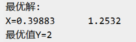
x y xy xy	y 2 y^2 y2
0.04998 0.04998 0.04998	1.57051 1.57051 1.57051
1 / 2 1/2 1/2	π / 2 \pi/2 π/2

The results are consistent with the predicted results.

• The optimal value varies with evolutionary algebra

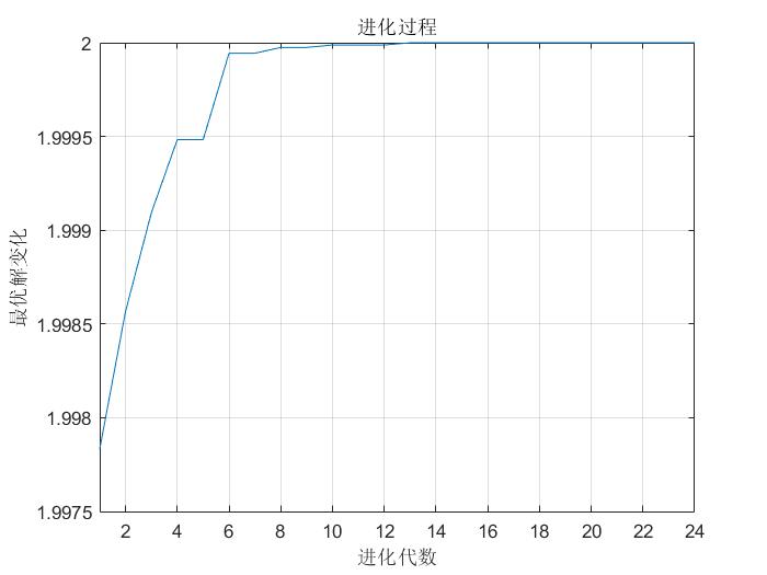
Here is just a simple example. Even without using multi population genetic algorithm, genetic algorithm alone can have better results. The focus is on the improvement of multi population algorithm to traditional genetic algorithm, and the specific problems should be analyzed in detail.

Code address

Full code in GitHub website Yes, if you have conditions, you can support it. Now pay attention to me. You're an old fan

Reference articles

Please refer to the following articles for the content of this article. If you have any questions, please contact this account

[1] Shi Feng. Analysis of 30 cases of MATLAB intelligent algorithm [M]. Beijing University of Aeronautics and Astronautics Press, 2011