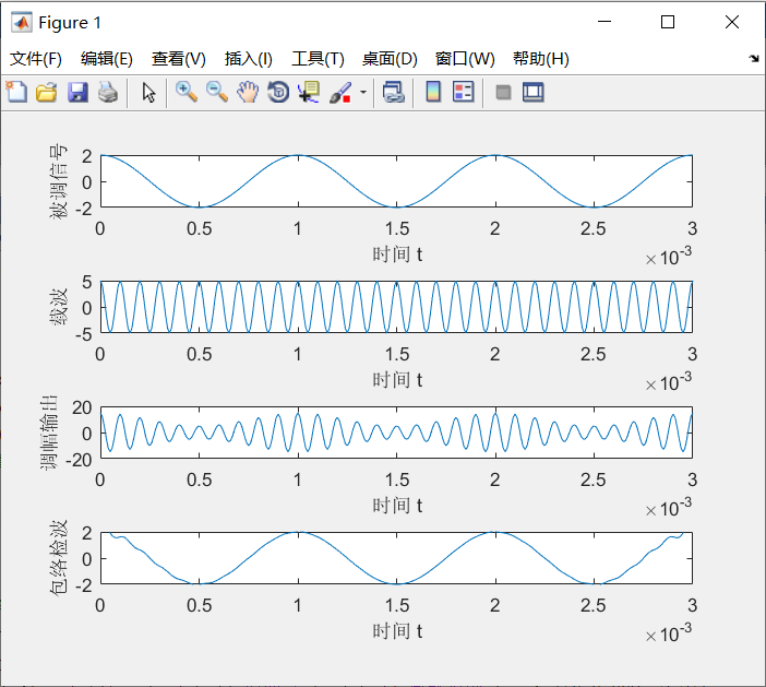
[example 2.1] try to simulate the input and output waveforms of an amplitude modulation system. Suppose that the input modulated signal is a cosine wave with an amplitude of 2v and a frequency of 1000Hz, the modulation system is 0.5, and the modulated carrier signal is a cosine wave with an amplitude of 5v and a frequency of 10KHz. The initial phase of all cosine waves is 0.

% ch2example1prg1.m
dt=1e-5;    % Simulation sampling interval
T=3*1e-3;   % Simulation end time
t=0:dt:T;
input=2*cos(2*pi*1000*t);       % Input modulated signal
carrier=5*cos(2*pi*1e4*t);      % carrier
output=(2+0.5*input).*carrier;  % Modulation output
% Mapping: Observe the input signal, carrier, And modulation output
subplot(4,1,1); plot(t,input);xlabel('time t');ylabel('Modulated signal');
subplot(4,1,2); plot(t,carrier);xlabel('time t');ylabel('carrier');
subplot(4,1,3); plot(t,output);xlabel('time t');ylabel('Am output');

% Noise free envelope detection and restoration of original signal
y = hilbert(output);
am = (abs(y)/5-2)*2;
subplot(4,1,4); plot(t,am);xlabel('time t');ylabel('Envelope detection');axis([0 0.003 -2 2]);

Simulation waveform of amplitude modulation displayed by real oscilloscope
In the program, the frequency of the input modulated signal is deliberately set to 1005Hz, so that the signal period is not an integral multiple of the simulation frame period. After operation, the "continuously" sliding modulated signal will be seen, the carrier shows phase jitter, and the received signal is contaminated with noise.

% ch2example1prg3.m
dt=1e-6;    % Simulation sampling interval
T=2*1e-3;   % Frame period of simulation
for N=0:500 % Total frames of simulation
    t=N*T+(0:dt:T);             % Sampling time in frame
    input=2*cos(2*pi*1005*t);   % Input the modulated signal, change 1005 to 1000, and you will not lose the dynamic graph.
    carrier=5*cos(2*pi*(1e4)*t+0.1*randn);  % carrier
    output=(2+0.5*input).*carrier;          % Modulation output
    noise=randn(size(t));       % Noise
    r=output+noise;             % Modulation signal through additive noise channel
    % Mapping: Observe the input signal, carrier, And modulation output
    subplot(3,1,1); plot([0:dt:T],input);xlabel('time t');
    ylabel('Modulated signal');text(T*2/3,1.5,['Current frames: N=',num2str(N)]);
    subplot(3,1,2); plot([0:dt:T],carrier);
    xlabel('time t');ylabel('carrier');
    subplot(3,1,3); plot([0:dt:T],r);
    xlabel('time t');ylabel('Am output');
    set(gcf,'DoubleBuffer','on');   % Double buffering to avoid drawing flicker
    drawnow;
end

[example 2.2] simulate the charging process of capacitor.

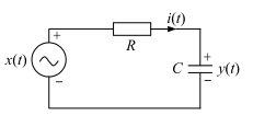
A voltage source charges the capacitor through a network of resistors connected in series with the capacitor. Let t = 0 be the initial time (before the initial time, the circuit is disconnected and does not work), the output voltage x(t) of the voltage source is the unit step function, the voltage at both ends of the capacitance is y(t), the circuit current is i(t), and the voltage source is regarded as the system input, and the voltage on the capacitance is regarded as the system output. The initial state of the circuit is y(0). Figure 2.3 shows the circuit diagram and the equivalent system model.

Set up circuit equations according to questions
y(t)=x(t)−Ri(t)i(t)=Cdy(t)dt \begin{aligned} y(t) &=x(t)-R i(t) \\ i(t) &=C \frac{\mathrm{d} y(t)}{\mathrm{d} t} \end{aligned} y(t)i(t)​=x(t)−Ri(t)=Cdtdy(t)​​

The simplification results in:

dy(t)dt=1RCx(t)−1RCy(t) \frac{\mathrm{d} y(t)}{\mathrm{d} t}=\frac{1}{R C} x(t)-\frac{1}{R C} y(t) dtdy(t)​=RC1​x(t)−RC1​y(t)

Substituting dy(t)=y(t+dt)-y(t) into the above formula, we can get:

y(t+dt)=y(t)+1RCx(t)dt−1RCy(t)dt y(t+\mathrm{d} t)=y(t)+\frac{1}{R C} x(t) \mathrm{d} t-\frac{1}{R C} y(t) \mathrm{d} t y(t+dt)=y(t)+RC1​x(t)dt−RC1​y(t)dt

Euler algorithm for differential equations
Δ≈dty(t+Δ)≈y(t)+1RCx(t)Δ−1RCy(t)Δ \Delta \approx \mathrm{d} t \\ y(t+\Delta) \approx y(t)+\frac{1}{R C} x(t) \Delta-\frac{1}{R C} y(t) \Delta Δ≈dty(t+Δ)≈y(t)+RC1​x(t)Δ−RC1​y(t)Δ

% ch2example2prg1.m
dt=1e-5;    % Simulation sampling interval
R=1e3;      % Resistance value
C=1e-6;     % Capacitance
T=5*1e-3;   % Simulation interval from -T reach +T
t=-T:dt:T;  % Computed discrete time series
y(1)=0;     % Initial value of capacitance voltage, It will remain unchanged when time is less than zero
            % If you want to simulate a zero input response, Set up y(1)=1 Equal nonzero value.
% ----Input signal setting:Selectable: Zero input,Step input,sinusoidal input,Square wave input, etc----
x=zeros(size(t));           % Initialize input signal storage matrix   
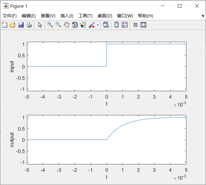
x=1*(t>=0);                 % The input signal jumps to 1 at 0, That is, the input is a step signal.
                            % If you want to simulate a zero input response, It can be set up here. x=0 that will do
% x=sin(2*pi*1000*t).*(t>=0);   % This is 1000 from zero Hz Sine signal of
% x=square(2*pi*500*t).*(t>=0); % This is 500 from zero Hz Square wave signal of
% Simulation start, Be careful: Circuit does not work before zero time, System state remains unchanged
for k=1:length(t)
    time=-T+k*dt;
    if time>=0 
        y(k+1)=y(k)+1./(R*C)*(x(k)-y(k))*dt; %Recursively solving the state value of the next simulation time
    else
        y(k+1)=y(k); % When the time is less than zero, the circuit is disconnected and the system does not work
    end
end
subplot(2,1,1);plot(t,x(1:length(t)));axis([-T T -1.1 1.1]);
xlabel('t');ylabel('input');
subplot(2,1,2);plot(t,y(1:length(t)));axis([-T T -1.1 1.1]);
xlabel('t');ylabel('output');