1. Theory introduction:  

        Zernike polynomial [1] (Netherlands) physical scientistFrits Zernike )Is a polynomial sequence defined on the unit circle and satisfying orthogonality, which can be written as:

Among them, Is the j-th Zernike mode, 0 ≤ r ≤ 1, 0 ≤ θ ≤ 2 π, m and N are the angular series and radial series of polynomials respectively, and m ≤ n is satisfied; When n − | m | is even, and radial polynomialDefined as:

2. Some properties of Zernike polynomials

2.1 Zernike polynomials are orthogonal, which can be written as follows:

2.2 the mean value of all orthogonal polynomials except the translation term (piston mode) is zero;

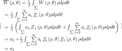
2.3 the mean value of each orthogonal polynomial (excluding piston mode) is 0; The proof is as follows (using property 2.1):

2.4 the mean wave front is equal to the coefficient of the translation term (piston mode)

2.5 each standard orthogonal polynomial has a minimum variance;

2.6 the wavefront variance is the sum of the squares of the coefficients of each polynomial, excluding the coefficients of the translation term;

Because of my limited ability, I can only do this.

So, is there a corresponding relationship between the j-th mode and n and M? The answer is yes. Generally, given any q, you can find the values of n and m. However, the values of n and m are related to the ranking of Zernike polynomials. The common ranking methods are Noll sequence (applied to atmospheric turbulence), OSA (human eye aberration) and Fringe. No matter how the ranking is, the value of Zernike polynomials is not required.

In addition, it should be noted that the polynomial is defined in the unit circle. In actual operation, a mask function needs to be added to shield the data outside the circle. Mainly, the data outside the circle is much larger than the data inside the circle.

3. Matlab simulation part:

3.1 define Noll sorting method

The values of j, m and n in Noll are as follows

about j = 1:20
j = [1, 2, 3, 4, 5, 6, 7, 8, 9,10,11,12,13,14,15,16,17,18,19,20]
NOLL Lower n and m The value of is:
m = [0, 1,-1, 0,-2, 2,-1, 1,-3, 3, 0, 2,-2, 4,-4, 1,-1, 3,-3, 5]
n = [0, 1, 1, 2, 2, 2, 3, 3, 3, 3, 4, 4, 4, 4, 4, 5, 5, 5, 5, 5]

and OSA The following values are:
m = [0,-1, 1,-2, 0, 2,-3,-1, 1, 3,-4,-2, 0, 2, 4,-5,-3,-1, 1, 3]
n = [0, 1, 1, 2, 2, 2, 3, 3, 3, 3, 4, 4, 4, 4, 4, 5, 5, 5, 5, 5]

Use code to realize Noll sorting, and return the values of n and m according to the sequence number j of Zernike polynomial:

function [n,m] = Noll_to_Zernike(j)
% Serial number j Start with 1; j = 1 For piston pattern
    if(j<1) 
        error('Noll indices start at 1.');
    end
    n  = 0;
    m  = 0;
    j1 = j-1;
    while (j1 > n)
        n  = n + 1;
        j1 = j1 - n;
        m  = (-1)^j * (mod(n,2) + 2*floor((j1+mod(n+1,2))/2));
    end
end

OSA sorting is realized by code, and the values of n and m are returned according to the sequence number j of Zernike polynomial

function [n,m] = OSA_to_Zernike(j)
 % Pay attention here j Starting from 0, j = 0 Corresponding to piston pattern,
 % If you want to start from, the parameters passed in are j-1，At this time, you can communicate with Noll_to_Zernike matching
     n = floor(sqrt(2*j+1)+0.5)-1;
     m = 2*j-n*(n+2);
end

3.2 main part of Zernike polynomial

function Znm= Zernike(j,res)
% parameter j:   Zernike Sequence number of polynomials
% parameter res: Zernike Polynomial resolution
    x           = linspace(-1,1,res);
    [x,y]       = meshgrid(x,x);
    [theta,rho] = cart2pol(x,y);% from(x,y)conversion(r,theta)

    [n,m]       = Noll_to_Zernike(j); % Call function, return n and m Value of
    % [n,m]     = OSA_to_Zernike(j-1)
    if m == 0
       deltam = 1;
    else
       deltam = 0;
    end
    Norm    = sqrt(2*(n+1)/(1+deltam));% Normalization factor 
    Rnm_rho = zeros(size(rho));        % Initialize radial polynomial
    for s = 0:(n-abs(m))/2
        Rnm_rho = Rnm_rho+(-1)^s.*prod(1:(n-s))*rho.^(n-2*s)/(prod(1:s)*...
        prod(1:((n+abs(m))/2-s))*prod(1:((n-abs(m))/2-s))); % Radial polynomial
    end
    if m < 0
       Znm = -Norm.*Rnm_rho.*sin(m.*theta); % m<0 Time zernike polynomial
    else
       Znm = Norm.*Rnm_rho.*cos(m.*theta);  % m>0 Time zernike polynomial
    end
    Znm = Znm.*(rho<=1); % mask = (rho<=1)，Only the data within the unit circle is retained
 end

3.3 main function

clc;clear all; close all
% Generate a pattern separately
res  = 60;                % The resolution is set to 60
Z    = Zernike(3,res);    % 3rd mode (astigmatism)
figure(1);imagesc(Z);colormap(jet);colorbar

% The first 60 modes are generated with a resolution of 60
num = 60;
Znm = zeros(res,res,num);
for i= 1:num
    Znm(:,:,i) = Zernike(i,60);
end
figure(5);imagesc(Znm(:,:,5));colormap(jet);colorbar

3.4 results section

After running the code, the image will appear.