1, Construction of decision tree
decision tree is a kind of common machine learning algorithm. It makes decisions based on tree structure. Step by step from the root node to the leaf node (decision). All data will eventually fall to leaf nodes, which can be classified or regressed.
Decision tree
Advantages: the calculation complexity is not high, the output result is easy to understand, is not sensitive to the loss of intermediate value, and can process irrelevant feature data.
Disadvantages: over matching may occur.
Applicable data types: numerical type and nominal type.
When constructing a decision tree, the first problem we need to solve is which feature on the current data set plays a decisive role in dividing data classification. In order to find the decisive features and divide the best results, we must evaluate each feature. After the test, the original data is divided into several data subsets. These data subsets are distributed on all branches of the first decision point. If the data under a branch belongs to the same type, the data set will be further divided here and correctly classified. If the data in the data subset does not belong to the same type, you need to repeat the process of dividing the data subset. The algorithm of how to divide the data subset is the same as that of the original data set, until all data with the same type are in one data subset.
General process of decision tree
(1) Collect data: any method can be used.
(2) Prepare data: the tree construction algorithm is only applicable to nominal data, so numerical data must be discretized.
(3) Analyze data: any method can be used. After constructing the tree, we should check whether the graph meets the expectations.
(4) Training algorithm: construct the data structure of the tree.
(5) Test algorithm: use the experience tree to calculate the error rate.
(6) Using algorithm: this step can be applied to any supervised learning algorithm, and using decision tree can better understand the internal meaning of data.
1. Information gain
The general principle of dividing data sets is to make disordered data more orderly
The change of information before and after dividing the data set is called information gain. Knowing how to calculate the information gain, we can calculate the information gain obtained by dividing the data set by each eigenvalue. The feature with the highest information gain is the best choice.
Before we can evaluate which data division method is the best data division, we must learn how to calculate the information gain. The measurement of set information is called Shannon entropy or entropy for short.
Entropy is defined as the expected value of information. Before clarifying this concept, we must know the definition of information. If the thing to be classified may be divided into multiple classifications, the symbol
x
i
x_i
xi's information is defined as
l
(
x
i
)
=
−
log
2
p
(
x
i
)
l(x_i) = -\log_2p(x_i)
l(xi)=−log2p(xi)
among
p
(
x
i
)
p(x_i)
p(xi) is the probability of selecting reclassification
In order to calculate entropy, we need to calculate the expected value of information contained in all possible values of all categories, which is obtained by the following formula:
H
=
−
∑
i
=
1
n
p
(
x
i
)
log
2
p
(
x
i
)
H = - \sum_{i = 1}^n p(x_i)\log_2p(x_i)
H=−i=1∑np(xi)log2p(xi)
Where n is the number of classifications.
When
p
(
x
i
)
=
0
p(x_i) = 0
p(xi) = 0 or
p
(
x
i
)
=
1
p(x_i) = 1
When p(xi) = 1,
H
=
0
H = 0
H=0, random variables have no uncertainty at all.
When
p
(
x
i
)
=
0.5
p(x_i) = 0.5
When p(xi) = 0.5,
H
=
1
H = 1
H=1, the uncertainty of random variables is the largest
Calculate Shannon entropy for a given dataset:
'''
Parameters:
    dataSet - data set
Returns:
    shannonEnt - Returns the Shannon entropy calculated for a given dataset
'''
def calcShannonEnt(dataSet):
    # Returns the number of rows in the dataset
    numEntries = len(dataSet)
    # Save a dictionary of the number of occurrences of each label
    labelCounts = {}
    # Each group of eigenvectors is counted
    for featVec in dataSet:
        # Extract label information
        currentLabel = featVec[-1]
        # If the label is not put into the dictionary of statistical times, add it
        if currentLabel not in labelCounts.keys():
            labelCounts[currentLabel] = 0
        # Label count
        labelCounts[currentLabel] += 1
    # Shannon entropy
    shannonEnt = 0.0
    # Calculate Shannon entropy
    for key in labelCounts:
        # The probability of selecting the label
        prob = float(labelCounts[key])/numEntries
        # Calculation of Shannon entropy by formula
        shannonEnt -= prob * log(prob, 2)
    # Return Shannon entropy
    return shannonEnt
First, calculate the total number of instances in the dataset. Then, create a data dictionary whose key value is the value of the last column. If the current key value does not exist, expand the dictionary and add the current key value to the dictionary. Each key value records the number of occurrences of the current category. Finally, the occurrence frequency of all class labels is used to calculate the probability of class occurrence. We will use this probability to calculate Shannon entropy and count the times of all class labels.
Marine biological data:
| Can we survive without coming to the surface | Are there fins | Belonging to fish | |
|---|---|---|---|
| 1 | yes | yes | yes |
| 2 | yes | yes | yes |
| 3 | yes | no | no |
| 4 | no | yes | no |
| 5 | no | yes | no |
Create a simple fish identification dataset from the table above
"""
Parameters:
    nothing
Returns:
    dataSet - data set
    labels - Classification properties
"""
def createDataSet():
    # data set
    dataSet = [[1, 1, 'yes'],
               [1, 1, 'yes'],
               [1, 0, 'no'],
               [0, 1, 'no'],
               [0, 1, 'no']]
    # Classification properties
    labels = ['no surfacing', 'flippers']
    # Return dataset and classification properties
    return dataSet, labels
if __name__ == '__main__':
    dataSet, labels = createDataSet()
    print(dataSet)
    print(calcShannonEnt(dataSet))
>>>
[[1, 1, 'yes'], [1, 1, 'yes'], [1, 0, 'no'], [0, 1, 'no'], [0, 1, 'no']]
0.9709505944546686
The higher the entropy, the more mixed data. We can add more classifications to the data set and observe how the entropy changes. Add a third category named may to test the change of entropy:
if __name__ == '__main__':
    dataSet, labels = createDataSet()
    dataSet[0][-1] = 'maybe'
    print(dataSet)
    print(calcShannonEnt(dataSet))
>>>
[[1, 1, 'maybe'], [1, 1, 'yes'], [1, 0, 'no'], [0, 1, 'no'], [0, 1, 'no']]
1.3709505944546687
The calculated entropy increases with the increase of classification. After obtaining the entropy, we can divide the data set according to the method of obtaining the maximum information gain.
2. Divide data sets
In addition to measuring the information entropy, the classification algorithm also needs to divide the data set and measure the entropy of the divided data set, so as to judge whether the data set is divided correctly. The information entropy is calculated once for the result of dividing the data set according to each feature, and then it is judged which feature is the best way to divide the data set.
Divide the data set according to the given characteristics:
"""
Parameters:
    dataSet - Data set to be divided
    axis - Characteristics of partitioned data sets
    value - The value of the feature to be returned
Returns:
    retDataSet - Partitioned dataset
"""
def splitDataSet(dataSet, axis, value):
    # Create a list of returned datasets
    retDataSet = []
    # Traversal dataset
    for featVec in dataSet:
        if featVec[axis] == value:
            # Remove axis feature
            reducedFeatVec = featVec[:axis]
            # Add eligible to the returned dataset
            reducedFeatVec.extend(featVec[axis + 1:])
            retDataSet.append(reducedFeatVec)
    # Returns the partitioned dataset
    return retDataSet
Test the function splitDataSet() on the previous simple sample data:
if __name__ == '__main__':
    dataSet, labels = createDataSet()
    print(dataSet)
    print(splitDataSet(dataSet, 0 ,1))
    print(splitDataSet(dataSet, 0 ,0))
>>>
[[1, 1, 'yes'], [1, 1, 'yes'], [1, 0, 'no'], [0, 1, 'no'], [0, 1, 'no']]
[[1, 'yes'], [1, 'yes'], [0, 'no']]
[[1, 'no'], [1, 'no']]
Next, traverse the entire data set, and cycle through the entropy and splitDataSet() function to find the best feature division method. Entropy calculation will tell us how to divide data sets is the best way to organize data.
Select the best data set division method:
"""
Parameters:
    dataSet - data set
Returns:
    bestFeature - Maximum information gain(optimal)Index value of the feature
"""
def chooseBestFeatureToSplit(dataSet):
    # Number of features
    numFeatures = len(dataSet[0]) - 1
    # Calculate Shannon entropy of data set
    baseEntropy = calcShannonEnt(dataSet)
    # information gain
    bestInfoGain = 0.0
    # Index value of optimal feature
    bestFeature = -1
    # Traverse all features
    for i in range(numFeatures):
        #Get the i th all features of dataSet
        featList = [example[i] for example in dataSet]
        # Create set set {}, elements cannot be repeated
        uniqueVals = set(featList)
        # Empirical conditional entropy
        newEntropy = 0.0
        # Calculate information gain
        for value in uniqueVals:
            # The subset of the subDataSet after partition
            subDataSet = splitDataSet(dataSet, i, value)
            # Calculate the probability of subsets
            prob = len(subDataSet) / float(len(dataSet))
            # The empirical conditional entropy is calculated according to the formula
            newEntropy += prob * calcShannonEnt(subDataSet)
        # information gain
        infoGain = baseEntropy - newEntropy
        # Print information gain for each feature
        print("The first%d The gain of each feature is%.3f" % (i, infoGain))
        # Calculate information gain
        if (infoGain > bestInfoGain):
            # Update the information gain to find the maximum information gain
            bestInfoGain = infoGain
            # Record the index value of the feature with the largest information gain
            bestFeature = i
    # Returns the index value of the feature with the largest information gain
    return bestFeature
if __name__ == '__main__':
    dataSet, labels = createDataSet()
    print(dataSet)
    print(chooseBestFeatureToSplit(dataSet))
>>>
[[1, 1, 'yes'], [1, 1, 'yes'], [1, 0, 'no'], [0, 1, 'no'], [0, 1, 'no']]
The gain of the 0th feature is 0.420
 The gain of the first feature is 0.171
0
The best index is 0, that is, the first feature is the best feature used to divide the dataset.
3. Recursive construction of decision tree
Working principle: get the original data set, and then divide the data set based on the best attribute value. Since there may be more than two eigenvalues, there may be data set division greater than two branches. After the first partition, the data will be passed down to the next node of the tree branch. On this node, we can partition the data again. Therefore, we can use the principle of recursion to deal with data sets.
The condition for the end of recursion: the program traverses all the attributes that divide the data set, or all instances under each branch have the same classification. If all instances have the same classification, a leaf node or termination block is obtained. Any data that reaches the leaf node must belong to the classification of the leaf node. If the dataset has processed all attributes, but the class label is still not unique, we need to decide how to define the leaf node. In this case, we usually use the majority voting method to determine the classification of the leaf node.
Majority vote:
"""
Parameters:
    classList - Class label list
Returns:
    sortedClassCount[0][0] - Elements that appear most here(Class label)
"""
def majorityCnt(classList):
    classCount = {}
    # Count the number of occurrences of each element in the classList
    for vote in classList:
        if vote not in classCount.keys():classCount[vote] = 0
        classCount[vote] += 1
    # Sort by dictionary values in descending order
    sortedClassCount = sorted(classCount.items(), key = operator.itemgetter(1), reverse = True)
    # Returns the most frequent element in the classList
    return sortedClassCount[0][0]
To create a decision tree:
"""
Parameters:
    dataSet - Training data set
    labels - Classification attribute label
Returns:
    myTree - Decision tree
"""
def createTree(dataSet, labels):
    # Take the classification label
    classList = [example[-1] for example in dataSet]
    # If all class labels are identical, the class label is returned directly
    if classList.count(classList[0]) == len(classList):
        return classList[0]
    # When all features are traversed, the class label with the most occurrences is returned
    if len(dataSet[0]) == 1:
        return majorityCnt(classList)
    # Select the optimal feature
    bestFeat = chooseBestFeatureToSplit(dataSet)
    # Optimal feature label
    bestFeatLabel = labels[bestFeat]
    # Label spanning tree based on optimal features
    myTree = {bestFeatLabel:{}}
    # Delete used feature labels
    del(labels[bestFeat])
    # The attribute values of all optimal features in the training set are obtained
    featValues = [example[bestFeat] for example in dataSet]
    # Remove duplicate attribute values
    uniqueVals = set(featValues)
    # Traverse the features and create a decision tree.
    for value in uniqueVals:
        # The class label is copied and stored in the new list variable subLabels
        subLabels = labels[:]
        myTree[bestFeatLabel][value] = createTree(splitDataSet(dataSet, bestFeat, value), subLabels)
    return myTree
Simple data set before testing
if __name__ == '__main__':
    dataSet, labels = createDataSet()
    print(dataSet)
    myTree = createTree(dataSet, labels)
    print(myTree)
>>>
[[1, 1, 'yes'], [1, 1, 'yes'], [1, 0, 'no'], [0, 1, 'no'], [0, 1, 'no']]
{'no surfacing': {0: 'no', 1: {'flippers': {0: 'no', 1: 'yes'}}}}
The variable myTree contains many nested dictionaries representing tree structure information. Starting from the left, the first keyword no surfacing is the feature name of the first partitioned dataset, and the value of this keyword is also another data dictionary. The second keyword is the data set divided by the no surfacing feature. The values of these keywords are the child nodes of the no surfacing node. These values may be class labels (such as' flippers') or another data dictionary. If the value is a class label, the child node is a leaf node; If the value is another data dictionary, the child node is a judgment node. This format structure repeats continuously to form the whole tree. This tree contains three leaf nodes and two judgment nodes.
2, Drawing a tree in Python using the Matplotlib annotation
1. Matplotlib
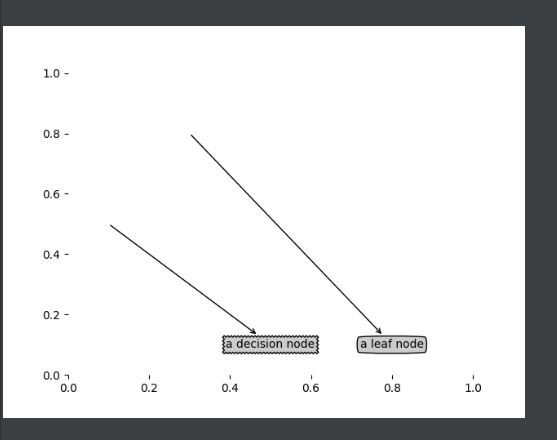
Draw tree nodes with text annotations:
# Define text box and arrow formats
decisionNode = dict(boxstyle="sawtooth", fc="0.8")
leafNode = dict(boxstyle="round4", fc="0.8")
arrow_args = dict(arrowstyle="<-")
"""
Parameters:
    nodeTxt - Node name
    centerPt - Text position
    parentPt - Arrow position of dimension
    nodeType - Node format
Returns:
    nothing
"""
def plotNode(nodeTxt, centerPt, parentPt, nodeType):
    createPlot.ax1.annotate(nodeTxt, xy=parentPt, xycoords='axes fraction',
                            xytext=centerPt, textcoords='axes fraction',
                            va="center", ha="center", bbox=nodeType, arrowprops=arrow_args)


def createPlot():
    fig = plt.figure(1, facecolor='white')
    fig.clf()
    createPlot.ax1 = plt.subplot(111, frameon=False)
    plotNode('a decision node', (0.5, 0.1), (0.1, 0.5), decisionNode)
    plotNode('a leaf node', (0.8, 0.1), (0.3, 0.8), leafNode)
    plt.show()
if __name__ == '__main__':
    createPlot()
Test effect:
2. Construct annotation tree
Although there are x and Y coordinates, how to place all tree nodes is a problem. You must know how many leaf nodes there are so that you can correctly determine the length of the x-axis; You also need to know how many layers the tree has so that you can correctly determine the height of the y-axis.
Get the number of leaf nodes and tree layers:
"""
Parameters:
    myTree - Decision tree
Returns:
    numLeafs - Number of leaf nodes of decision tree
"""
def getNumLeafs(myTree):
    # Initialize leaf
    numLeafs = 0
    #myTree.keys() in Python 3 returns dict_keys, not a list,
    #Therefore, you cannot use the method of myTree.keys()[0] to obtain node properties. You can use list(myTree.keys())[0]
    firstStr = next(iter(myTree))
    # Get the next set of dictionaries
    secondDict = myTree[firstStr]
    for key in secondDict.keys():
        # Test whether the node is a dictionary. If it is not a dictionary, it means that the node is a leaf node
        if type(secondDict[key]).__name__=='dict':
            numLeafs += getNumLeafs(secondDict[key])
        else:   numLeafs +=1
    return numLeafs

"""
Parameters:
    myTree - Decision tree
Returns:
    maxDepth - Layers of decision tree
"""
def getTreeDepth(myTree):
    # Initialize decision tree depth
    maxDepth = 0
    #myTree.keys() in Python 3 returns dict_keys, not a list,
    #Therefore, you cannot use the method of myTree.keys()[0] to obtain node properties. You can use list(myTree.keys())[0]
    firstStr = next(iter(myTree))
    # Get next dictionary
    secondDict = myTree[firstStr]
    for key in secondDict.keys():
        #Test whether the node is a dictionary. If it is not a dictionary, it means that the node is a leaf node
        if type(secondDict[key]).__name__=='dict':
            thisDepth = 1 + getTreeDepth(secondDict[key])
        else:   thisDepth = 1
        # Update layers
        if thisDepth > maxDepth: maxDepth = thisDepth
    return maxDepth
The function retrieveTree outputs the pre stored tree information, avoiding the trouble of creating a tree from the data every time you test the code.
def retrieveTree(i):
    """
    Predefined tree structure for testing
    """
    listOfTrees = [{'no surfacing': {0: 'no', 1: {'flippers': {0: 'no', 1: 'yes'}}}},
                   {'no surfacing': {0: 'no', 1: {'flippers': {0: {'head': {0: 'no', 1: 'yes'}}, 1: 'no'}}}}
                  ]
    return listOfTrees[i]
if __name__ == '__main__':
    print(retrieveTree(1))
    myTree = retrieveTree(0)
    print(getNumLeafs(myTree))
    print(getTreeDepth(myTree))
>>>
{'no surfacing': {0: 'no', 1: {'flippers': {0: {'head': {0: 'no', 1: 'yes'}}, 1: 'no'}}}}
3
2
Both the getNumLeafs() function and the gettreedepts() function returned the correct results. Next, draw a complete tree.
Dimension directed edge attribute values:
"""
Parameters:
    cntrPt,parentPt - Used to calculate dimension locations
    txtString - Marked content
Returns:
    nothing
"""
def plotMidText(cntrPt, parentPt, txtString):
    xMid = (parentPt[0]-cntrPt[0])/2.0 + cntrPt[0]#Calculate dimension location
    yMid = (parentPt[1]-cntrPt[1])/2.0 + cntrPt[1]
    createPlot.ax1.text(xMid, yMid, txtString, va="center", ha="center", rotation=30)
Draw decision tree:
"""
Parameters:
    myTree - Decision tree(Dictionaries)
    parentPt - Marked content
    nodeTxt - Node name
Returns:
    nothing
"""
def plotTree(myTree, parentPt, nodeTxt):
    # Set node format
    decisionNode = dict(boxstyle="sawtooth", fc="0.8")
    # Format leaf nodes
    leafNode = dict(boxstyle="round4", fc="0.8")
    # Get the number of decision leaf nodes, which determines the width of the tree
    numLeafs = getNumLeafs(myTree)
    # Get the number of decision tree layers
    depth = getTreeDepth(myTree)
    # Next dictionary
    firstStr = next(iter(myTree))
    # Center position
    cntrPt = (plotTree.xOff + (1.0 + float(numLeafs))/2.0/plotTree.totalW, plotTree.yOff)
    # Dimension directed edge attribute values
    plotMidText(cntrPt, parentPt, nodeTxt)
    # Draw node
    plotNode(firstStr, cntrPt, parentPt, decisionNode)
    # The next dictionary is to continue drawing child nodes
    secondDict = myTree[firstStr]
    # y offset
    plotTree.yOff = plotTree.yOff - 1.0/plotTree.totalD
    for key in secondDict.keys():
        # Test whether the node is a dictionary. If it is not a dictionary, it means that the node is a leaf node, not a leaf node. Call recursively to continue drawing
        if type(secondDict[key]).__name__=='dict':
            plotTree(secondDict[key],cntrPt,str(key))
        # If it is a leaf node, draw the leaf node and mark the directed edge attribute value
        else:
            plotTree.xOff = plotTree.xOff + 1.0/plotTree.totalW
            plotNode(secondDict[key], (plotTree.xOff, plotTree.yOff), cntrPt, leafNode)
            plotMidText((plotTree.xOff, plotTree.yOff), cntrPt, str(key))
    plotTree.yOff = plotTree.yOff + 1.0/plotTree.totalD
To create a paint panel:
"""
Parameters:
    inTree - Decision tree(Dictionaries)
Returns:
    nothing
"""
def createPlot(inTree):
    # Create fig
    fig = plt.figure(1, facecolor='white')
    # Empty fig
    fig.clf()
    axprops = dict(xticks=[], yticks=[])
    # Remove the x and y axes
    createPlot.ax1 = plt.subplot(111, frameon=False, **axprops)
    # Get the number of decision nodes
    plotTree.totalW = float(getNumLeafs(inTree))
    # Get the number of decision tree layers
    plotTree.totalD = float(getTreeDepth(inTree))
    # x offset
    plotTree.xOff = -0.5/plotTree.totalW; plotTree.yOff = 1.0;
    # Draw decision tree
    plotTree(inTree, (0.5,1.0), '')
    # Display drawing results
    plt.show()
if __name__ == '__main__':
    myTree = retrieveTree(0)
    createPlot(myTree)

3, Test and store classifiers
1. Test algorithm: use decision tree to perform classification
After constructing the decision tree based on the training data, we can use it to classify the actual data. When performing data classification, the decision tree and the label vector used to construct the tree are needed. Then, the program compares the test data with the values on the decision tree, and recursively executes the process until it enters the leaf node; Finally, the test data is defined as the type of leaf node.
Use the classification function of the decision tree:
"""
Parameters:
    inputTree - Generated decision tree
    featLabels - Store the selected optimal feature label
    testVec - Test data list, the order corresponds to the optimal feature label
Returns:
    classLabel - Classification results
"""
def classify(inputTree, featLabels, testVec):
    # Get decision tree node
    firstStr = next(iter(inputTree))
    # Next dictionary
    secondDict = inputTree[firstStr]
    featIndex = featLabels.index(firstStr)
    for key in secondDict.keys():
        if testVec[featIndex] == key:
            if type(secondDict[key]).__name__ == 'dict':
                classLabel = classify(secondDict[key], featLabels, testVec)
            else: classLabel = secondDict[key]
    return classLabel
if __name__ == '__main__':
    dataSet, labels = createDataSet()
    print(labels)
    myTree = retrieveTree(0)
    print(myTree)
    print(classify(myTree, labels, [1, 0]))
    print(classify(myTree, labels, [1, 1]))
>>>
['no surfacing', 'flippers']
{'no surfacing': {0: 'no', 1: {'flippers': {0: 'no', 1: 'yes'}}}}
no
yes
2. Use algorithm: storage of decision tree
Constructing a decision tree is a time-consuming task. It takes several seconds to process a small data set, such as the previous sample data. If the data set is large, it will consume a lot of computing time. However, using the created decision tree to solve the classification problem can be completed quickly. Therefore, in order to save computing time, it is best to call the constructed decision tree every time the classification is executed.
Storage decision tree:
"""
Parameters:
    inputTree - Generated decision tree
    filename - Storage file name of the decision tree
Returns:
    nothing
"""
def storeTree(inputTree, filename):
    with open(filename, 'wb') as fw:
        pickle.dump(inputTree, fw)
Read decision tree:
"""
Parameters:
    filename - Storage file name of the decision tree
Returns:
    pickle.load(fr) - Decision tree dictionary
"""
def grabTree(filename):
    fr = open(filename, 'rb')
    return pickle.load(fr)
if __name__ == '__main__':
    myTree = retrieveTree(0)
    storeTree(myTree, 'classifierStorage.txt')
    grabTree('classifierStorage.txt')

Through the above code, we can store the classifier on the hard disk instead of learning it again every time we classify the data, which is also one of the advantages of the decision tree.
4, Using decision tree to predict vehicle condition
The condition of the vehicle is divided into four categories:
- unacc (Unacceptable condition is very poor)
- acc (Acceptable condition is normal)
- good (Good)
- vgood (Very good)
Judge the condition of the vehicle through the following classification attributes:
- buying (purchase price: vhigh, high, med, low)
- maint (maintenance price: vhigh, high, med, low)
- Doors (several doors: 2, 3, 4, 5more)
- persons (capacity: 2, 4, more)
- lug_boot (storage space: small, med, big)
- safety: low, Med, high
Data sample:
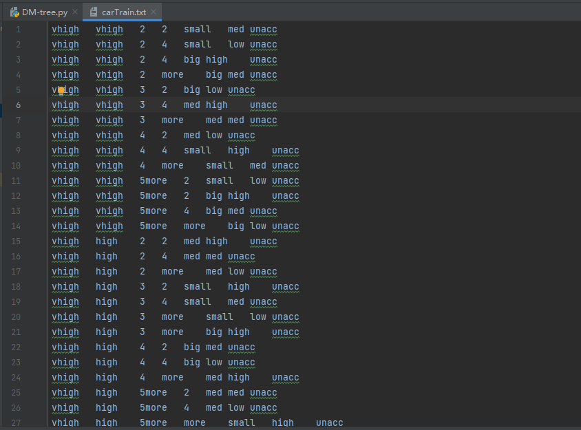
Test code:
if __name__ == '__main__':
    fr = open('carTrain.txt')
    cars = [inst.strip().split('\t') for inst in fr.readlines()]
    carLabels = ['buying', 'maint', 'doors', 'persons', 'lub_boot', 'safety']
    carsTree = createTree(cars, carLabels)
    print(carsTree)
    createPlot(carsTree)
Test results:
>>>
{'safety': {'low': 'unacc', 'med': {'persons': {'2': 'unacc', '4': {'buying': {'low': {'maint': {'low': 'acc', 'med': 'good', 'high': 'acc', 'vhigh': 'acc'}}, 'med': {'maint': {'low': 'acc', 'med': 'acc', 'high': 'unacc', 'vhigh': 'acc'}}, 'high': {'maint': {'low': 'unacc', 'med': 'acc', 'high': 'unacc', 'vhigh': 'unacc'}}, 'vhigh': {'maint': {'low': 'unacc', 'med': 'acc', 'high': 'unacc', 'vhigh': 'unacc'}}}}, 'more': {'buying': {'low': {'maint': {'med': {'doors': {'2': 'good', '3': 'good', '4': 'acc'}}, 'vhigh': {'doors': {'2': 'acc', '3': 'acc', '4': 'unacc'}}}}, 'med': {'doors': {'2': 'acc', '3': 'acc', '4': {'maint': {'med': 'acc', 'vhigh': 'unacc'}}}}, 'high': {'maint': {'med': {'doors': {'2': 'acc', '3': 'acc', '4': 'unacc'}}, 'vhigh': 'unacc'}}, 'vhigh': {'maint': {'med': {'doors': {'2': 'acc', '3': 'acc', '4': 'unacc'}}, 'vhigh': 'unacc'}}}}}}, 'high': {'persons': {'4': {'buying': {'low': {'maint': {'med': {'doors': {'2': 'vgood', '3': 'good', '4': 'good'}}, 'vhigh': 'acc'}}, 'med': {'doors': {'2': {'maint': {'med': 'vgood', 'vhigh': 'acc'}}, '3': 'acc', '4': 'acc'}}, 'high': {'maint': {'med': 'acc', 'vhigh': 'unacc'}}, 'vhigh': {'maint': {'med': 'acc', 'vhigh': 'unacc'}}}}, '2': 'unacc', 'more': {'buying': {'low': {'doors': {'4': 'vgood', '3': 'vgood', '5more': {'maint': {'low': 'good', 'high': 'acc'}}}}, 'med': {'maint': {'low': {'doors': {'4': 'vgood', '3': 'vgood', '5more': 'good'}}, 'high': 'acc'}}, 'high': 'acc', 'vhigh': {'maint': {'low': 'acc', 'high': 'unacc'}}}}}}}}

Along different branches of the decision tree, the condition of the vehicle can be judged by some attributes of the vehicle itself.
The decision tree matches the experimental data very well, but there may be too many matching options. This problem is called over matching. In order to reduce the over matching problem, we can cut the decision tree and remove some unnecessary leaf nodes. If a leaf node can only add a little information, it can be deleted and incorporated into other leaf nodes. ID3 algorithm cannot directly process numerical data. Although we can convert numerical data into nominal data by quantitative method, if there are too many feature divisions, ID3 algorithm will still face other problems.
5, Improved algorithm
1. C4.5 algorithm
C4.5 algorithm is a classical algorithm used to generate decision tree. It is an extension and optimization of ID3 algorithm. C4.5 algorithm improves ID3 algorithm. The main improvements are:
- Using information gain rate to select partition features overcomes the deficiency of using information gain, but the information gain rate has a preference for attributes with a small number of values;
- It can handle discrete and continuous attribute types, that is, discrete continuous attributes;
- Capable of processing training data with missing attribute values;
- Pruning during tree construction;
Information gain rate
The information gain criterion has a preference for attributes with a large number of values. In order to reduce the possible adverse effects of this preference, C4.5 algorithm uses the information gain rate to select the optimal partition attributes. Gain rate formula:
G
a
i
n
_
r
a
t
i
o
(
D
,
a
)
=
G
a
i
n
(
D
,
a
)
I
V
(
a
)
Gain\_ratio(D,a) = \frac{ Gain(D,a)}{IV(a)} \quad
Gain_ratio(D,a)=IV(a)Gain(D,a)
among
I
V
(
a
)
=
−
∑
v
=
1
V
∣
D
v
∣
∣
D
∣
log
2
∣
D
v
∣
∣
D
∣
IV(a) = -\sum_{v=1}^V \frac{|D^v|}{|D|}\log_2 \frac{|D^v|}{|D|} \quad \quad
IV(a)=−v=1∑V∣D∣∣Dv∣log2∣D∣∣Dv∣
It is called the "intrinsic value" of attribute A. The more possible values of attribute a (i.e. the greater V), the
I
V
(
a
)
IV(a)
The larger the value of IV(a) is usually
The information gain rate criterion has a preference for attributes with a small number of values. Therefore, C4.5 algorithm does not directly select the candidate partition attribute with the largest information gain rate, but first find the attribute with higher information gain than the average level from the candidate partition attributes, and then select the attribute with the highest information gain rate.
Processing of continuous features
When the attribute type is discrete, there is no need to discretize the data;
When the attribute type is continuous, the data needs to be discretized. The specific ideas are as follows:
Specific ideas:
The continuous characteristic a of M samples has m values, arranged from small to large
a
1
,
a
2
,
...
,
a
n
a_1,a_2,{\ldots} ,a_n
a1, a2,..., an, take the average of two adjacent sample values as the division point, there are m-1 in total, and the ith division point Ti is expressed as:
T
i
=
(
a
i
+
a
i
+
1
)
/
2
T_i = (a_i + a_{i+1})/2
Ti=(ai+ai+1)/2 .
The information gain rate when these m-1 points are used as binary segmentation points is calculated respectively. The point with the largest information gain rate is selected as the best segmentation point of the continuous feature. For example, the point with the largest information gain rate is
a
t
a_t
at, then less than
a
t
a_t
The value of at is category 1, greater than
a
t
a_t
The value of at is class 2, so the discretization of continuous features is achieved.
2. CART
CART algorithm constructs a decision tree for classification: the size of Gini index is used to measure the advantages and disadvantages of each partition point.
The definition of Gini index is: in the classification problem, assuming that D has k classes, the probability that the sample point belongs to class k is
p
k
p_k
pk, then the probability
The Gini value of the distribution is defined as:
G
i
n
i
(
D
)
=
∑
k
=
1
K
p
k
(
1
−
p
k
)
=
1
−
∑
k
=
1
K
p
k
2
Gini(D) = \sum_{k=1}^K p_k(1 - p_k) = 1 - \sum_{k=1}^K p_k^2
Gini(D)=k=1∑Kpk(1−pk)=1−k=1∑Kpk2
G
i
n
i
(
D
)
Gini(D)
The smaller Gini(D), the higher the purity of data set D;
Given dataset D, the Gini index of attribute a is defined as:
G
i
n
i
i
n
d
e
x
(
D
,
a
)
=
∑
v
=
1
V
∣
D
v
∣
∣
D
∣
G
i
n
i
(
D
v
)
Gini_index(D,a) = \sum_{v=1}^V \frac{|D^v|}{|D|}Gini(D^v) \quad
Giniindex(D,a)=v=1∑V∣D∣∣Dv∣Gini(Dv)
In the candidate attribute set A, select the attribute that minimizes the Gini index after partition as the optimal partition attribute.