1. Linear relationship model
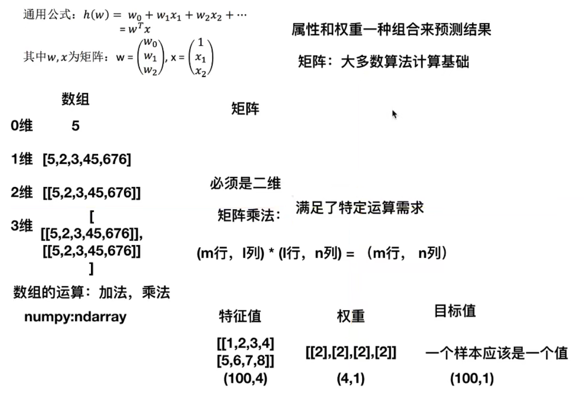
A function that predicts through a linear combination of attributes:
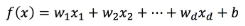
w is the weight, b is the offset term, which can be understood as:
2. Linear regression (iteration, self-learning)
Definition: linear regression is a regression analysis modeled between one or more independent variables and dependent variables. It can be a linear combination between one or more independent variables (a kind of linear regression)
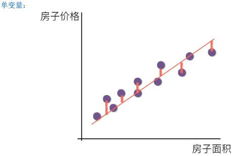
Univariate linear regression: only one variable (only one eigenvalue) is involved
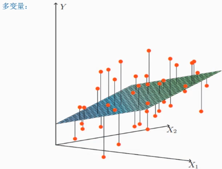
Multiple linear regression: involving two or more variables (multiple eigenvalues)
Formula:
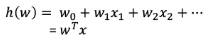
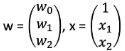
Where W and X are matrices:
3. Matrix operation (linear regression operation)
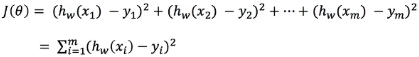
4. Loss function strategy (error size)
●  Is the true value of the ith training sample
●  It is the combined prediction function of the eigenvalues of the ith training sample
Definition of total loss (least square method):
The purpose is to reduce this loss
How to find w in the model to minimize the loss? (the purpose is to find the W value corresponding to the minimum loss)
(optimization method) solution 1: normal equation of least square method:
Solution: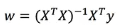
X is the eigenvalue matrix and y is the target value matrix
Disadvantages: when the features are too complex, the solution speed is too slow
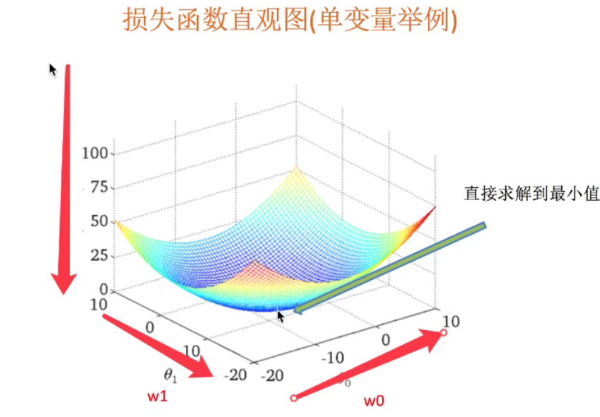
(optimization method) solution 2: gradient descent of least square method (important)
Take W0 and W1 in a single variable as an example:
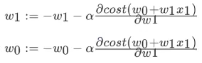
α The learning rate needs to be specified manually,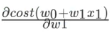 Indicates the direction
Understanding: follow the descending direction of this function to find the lowest point of the valley, and then update the W value
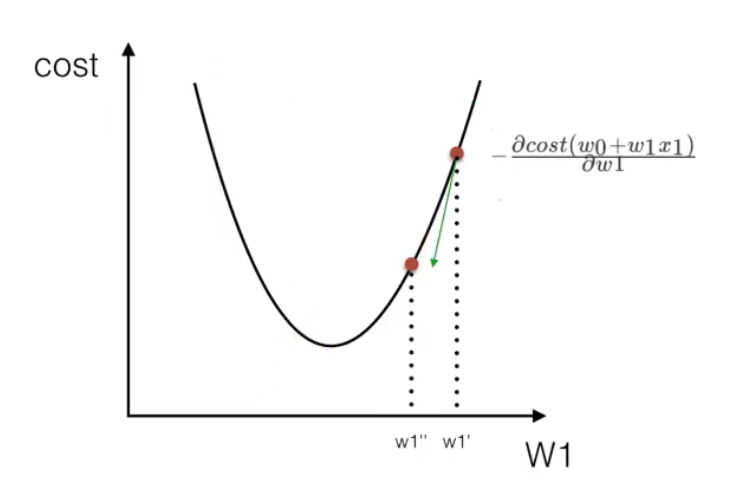
Usage: facing the task of huge training data scale
5.sklearn linear regression normal equation, gradient descent API
● sklearn.linear_model.LinearRegression -- normal equation
● ordinary least squares linear regression
● coef_: regression coefficient
● sklean.linear_ Model.sgdrepression -- gradient descent
● minimize the linear model by using SGD
● coef_: regression coefficient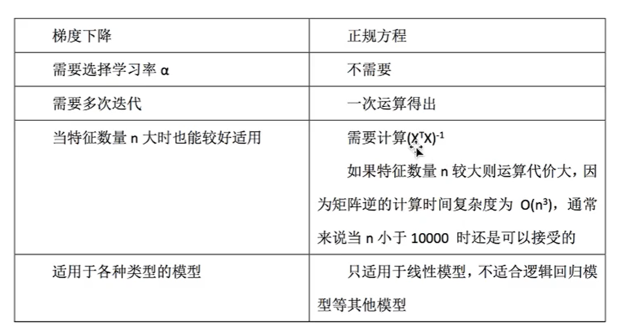
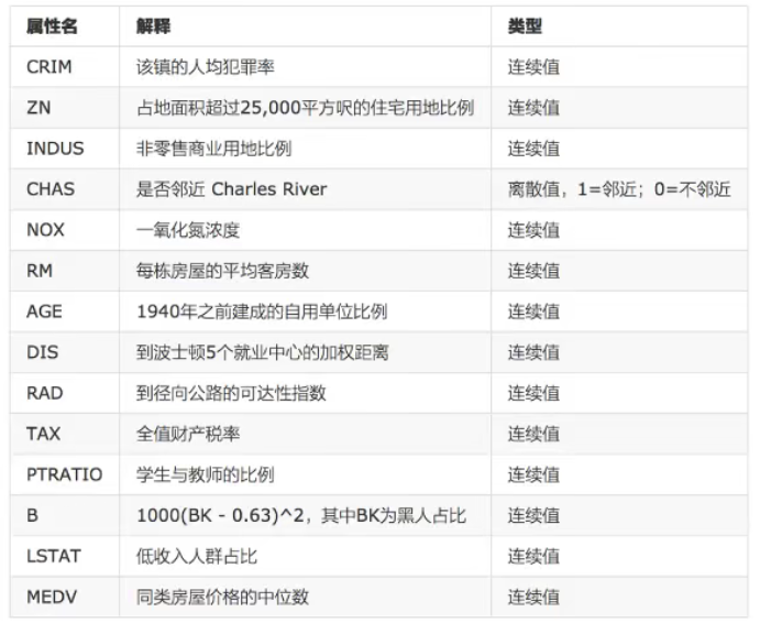
6. Linear regression example - Boston house price forecast
House price characteristics:
Boston house price data set analysis process:
1. Boston area house price data acquisition
2. Boston area house price data segmentation
3. Standardized processing of training and test data
4. The simplest linear regression model linear regression and gradient descent estimation SGDRegression are used to predict house prices
demo:
from sklearn.datasets import load_boston
from sklearn.linear_model import LinearRegression, SGDRegressor
from sklearn.model_selection import train_test_split
from sklearn.preprocessing import StandardScaler
from sklearn.metrics import mean_squared_error
def mylinear():
"""
Linear regression prediction of house price
:return: None
"""
# get data
lb = load_boston()
# The data is divided into training set and test set
x_train, x_test, y_train, y_test = train_test_split(lb.data, lb.target, test_size=0.25)
# print(y_train,y_test)
# Carry out standardization processing, and standardize the eigenvalue and target values respectively
# Eigenvalue standardization
std_x = StandardScaler()
x_train = std_x.fit_transform(x_train)
x_test = std_x.transform(x_test)
# Target value standardization, y_ train,y_ The test format is one-dimensional, and the standard scaler requires two-dimensional, so reshape the shape with reshape
std_y = StandardScaler()
y_train = std_y.fit_transform(y_train.reshape(-1,1))
y_test = std_y.transform(y_test.reshape(-1,1))
#Algorithm model
#Solution of normal equation and prediction results
lr = LinearRegression()
lr.fit(x_train,y_train)
print(lr.coef_)
#Forecast test set house price
y_lr_predict = std_y.inverse_transform(lr.predict(x_test))
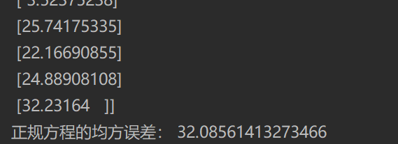
print("The predicted price of each house in the normal equation test set:",y_lr_predict)
print("Mean square error of normal equation:",mean_squared_error(std_y.inverse_transform(y_test),y_lr_predict))
#gradient descent
sgd = SGDRegressor()
sgd.fit(x_train, y_train)
print(sgd.coef_)
# Forecast test set house price
y_sgd_predict = std_y.inverse_transform(sgd.predict(x_test))
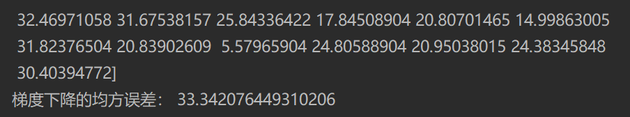
print("Forecast price of each house in the test set:", y_sgd_predict)
print("Mean square error of gradient descent:", mean_squared_error(std_y.inverse_transform(y_test), y_sgd_predict))
return None
if __name__ == "__main__":
mylinear()
Operation results:
Regression performance evaluation:
(mean square error (MSE) evaluation mechanism:
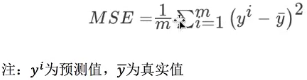
● mean_squared_error(y_true,y_pred)
● mean square error regression loss
● y_true: true value
● y_pred: predicted value
● return: floating point number result
Note: the real value and the predicted value are the values before standardization
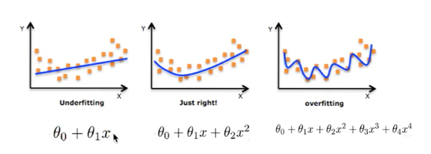
7. Over fitting and under fitting
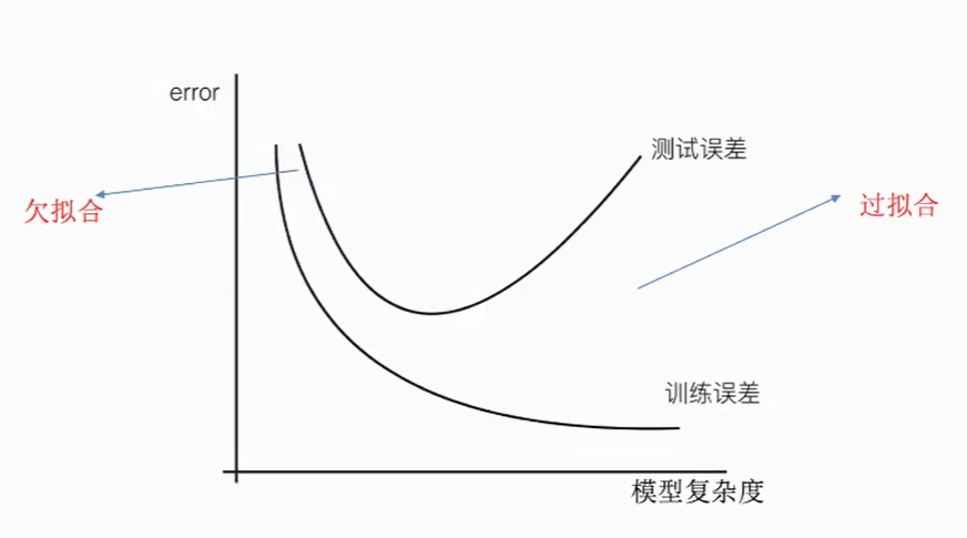
Over fitting: a hypothesis can get better fitting than other hypotheses on the training data, but it can not fit the data well on the data set outside the training data. At this time, it is considered that this hypothesis has over fitting phenomenon. (the model is too complex)
Under fitting: a hypothesis can not get better fitting on the training data, but it can not fit the data well on the data set other than the training data. At this time, it is considered that this hypothesis has the phenomenon of under fitting. (the model is too simple)
Causes and solutions of under fitting:
● cause: too few characteristics of data are learned
● Solution: increase the number of features of the data
Over fitting causes and Solutions
● Reason: there are too many original features and some noisy features. The model is too complex because the model tries to take into account all test data points
● Solution: select features and eliminate features with high relevance (it is difficult to do); Cross validation (make all data trained); Regularization
L2 regularization:
Function: it can make each element of W very small and close to 0
Advantages: the smaller the parameter, the simpler the model, and the simpler the model, the less likely it is to produce over fitting.
8. Ridge regression - linear regression with L2 regularization
● sklean.linear_model.Ridge(alpha=1.0)
● linear least squares with I2 regularization
● alpha: regularization strength λ 0~1 1~10
● coef_: regression coefficient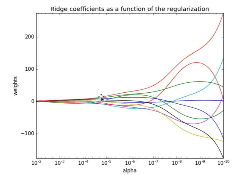
Note: it will not be equal to 0, but will be infinitely close to 0
demo:
from sklearn.datasets import load_boston
from sklearn.linear_model import LinearRegression, SGDRegressor,Ridge
from sklearn.model_selection import train_test_split
from sklearn.preprocessing import StandardScaler
from sklearn.metrics import mean_squared_error
def ridge():
"""
Linear regression prediction of house price
:return: None
"""
# get data
lb = load_boston()
# The data is divided into training set and test set
x_train, x_test, y_train, y_test = train_test_split(lb.data, lb.target, test_size=0.25)
# print(y_train,y_test)
# Carry out standardization processing, and standardize the eigenvalue and target values respectively
# Eigenvalue standardization
std_x = StandardScaler()
x_train = std_x.fit_transform(x_train)
x_test = std_x.transform(x_test)
# Target value standardization, y_ train,y_ The test format is one-dimensional, and the standard scaler requires two-dimensional, so reshape the shape with reshape
std_y = StandardScaler()
y_train = std_y.fit_transform(y_train.reshape(-1,1))
y_test = std_y.transform(y_test.reshape(-1,1))
#Algorithm model
#Ridge regression
rd = Ridge(alpha=1.0)
rd.fit(x_train, y_train)
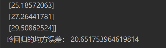
print(rd.coef_)
# Forecast test set house price
y_rd_predict = std_y.inverse_transform(rd.predict(x_test))
print("Forecast price of each house in the test set:", y_rd_predict)
print("Mean square error of ridge regression:", mean_squared_error(std_y.inverse_transform(y_test), y_rd_predict))
return None
if __name__ == "__main__":
ridge()
Operation results:
Comparison between linear regression and ridge regression:
● ridge regression: the regression coefficient obtained by regression is more practical and reliable. In addition, it can make the fluctuation range of estimation parameters smaller and more stable. It has great practical value in the research of too many morbid data.
9. Classification algorithm - logistic regression (Solving binary classification problem)
Logistic regression formula:
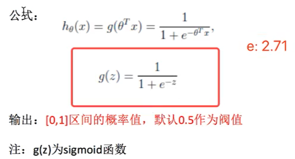
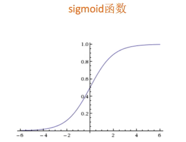
Activation function Sigmoid: regression to classification
10. Logistic regression loss function and optimization
It is the same as the principle of linear regression, but because it is a classification problem, the loss function is different and can only be solved by gradient descent
Log likelihood loss function:
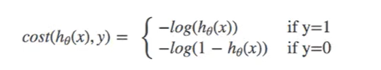
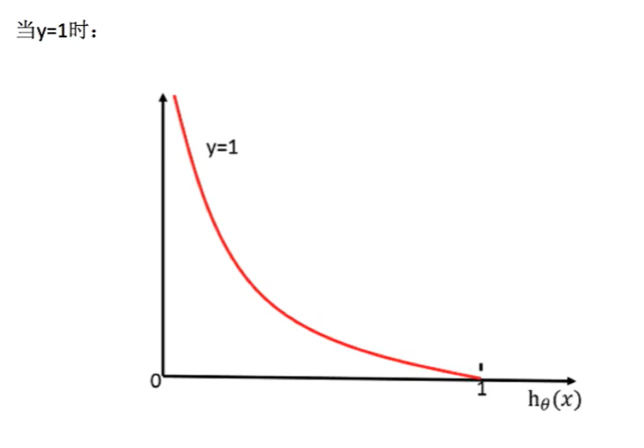
Complete loss function:
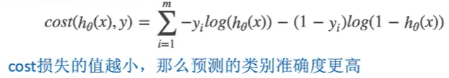
When y = 1 When, the classification result is 1 (positive): (horizontal axis classification result, vertical axis loss function)
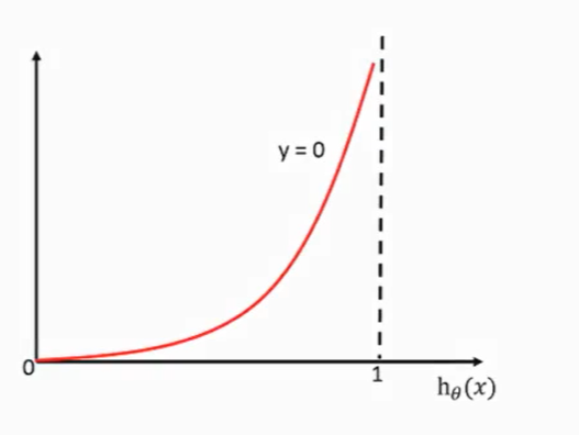
When y = 0 When, the classification result is 0 (negative): (horizontal axis classification result, vertical axis loss function)
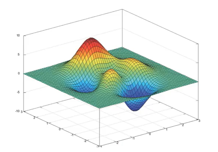
The log likelihood loss may fall into the local optimal solution (the mean square error has only one value and there is no local optimal problem):
11. Logistic regression API
● sklearn.lnear_model.LogisticRegression(penal='l2',C=1.0)
● Logistic regression classifier
● coef_: regression coefficient
12. Logistic regression cases
Data address: https://archive.ics.uci.edu/ml/machine-learning-databases/
demo:
#Model API
from sklearn.linear_model import LogisticRegression
#Recall API
from sklearn.metrics import classification_report
#Split dataset API
from sklearn.model_selection import train_test_split
#Standardized API
from sklearn.preprocessing import StandardScaler
import pandas as pd
import numpy as np


def logistic():
    """
    Logistic regression classification for tumor prediction
    :return:    None
    """
    # Construct column label name
    column = ['Sample code number', 'Clump Thickness',
              'Uniformity of Cell Size', 'Uniformity of Cell Shape', 'Marginal Adhesion',
              'Single Epithelial Cell Size', 'Bare Nuclei', 'Bland Chromatin',
              'Normal Nucleoli', 'Mitoses', 'Class']
    # Read data
    data = pd.read_csv("https://archive.ics.uci.edu/ml/machine-learning-databases/"
                       "breast-cancer-wisconsin/breast-cancer-wisconsin.data", names=column)
    # print(data)

    #Handling of missing values
    data = data.replace(to_replace="?",value=np.nan)
    #Delete missing values
    data = data.dropna()
    #Dataset segmentation
    x_train, x_test, y_train, y_test = train_test_split(data[column[1:10]], data[column[10]], test_size=0.25)
    #Standardized treatment
    std = StandardScaler()
    x_train = std.fit_transform(x_train)
    x_test = std.transform(x_test)
    #Logistic regression prediction
    lg = LogisticRegression(C=1.0)
    lg.fit(x_train,y_train)
    print(lg.coef_)
    print("Prediction accuracy:",lg.score(x_test,y_test))
    #recall
    y_predict = lg.predict(x_test)
    print("Recall rate:",classification_report(y_test,y_predict,labels=[2,4],target_names=["Benign","malignant"]))
    return None


if __name__ == "__main__":
    logistic()
Operation results:
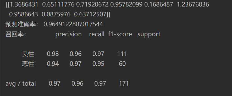
Summary (II Classification questions):
Application: advertising click through rate prediction, whether it is sick, financial fraud, whether it is a false account
Advantages: it is suitable for scenes where a classification probability needs to be obtained. It is simple and fast
Disadvantages: it is difficult to deal with multi classification problems
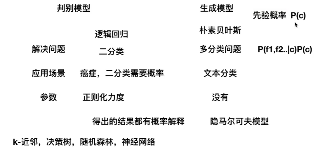
13. Generation model and discrimination model
The criterion of the two is whether there is a priori probability
14. Unsupervised learning K-means clustering algorithm
Algorithm flow:
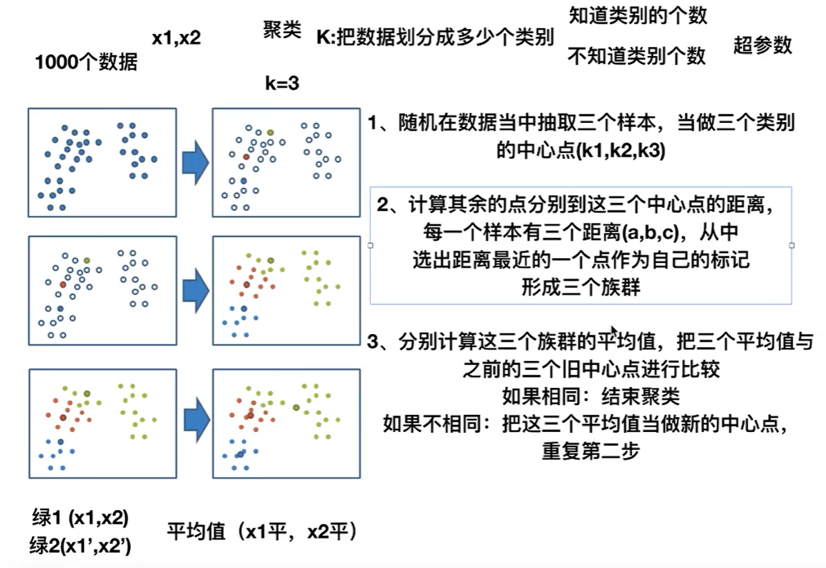
Steps:
1. K points in the feature space are randomly set as the initial clustering center
2. For each other point, calculate the distance to K centers. For unknown points, select the nearest cluster center as the marker category
3. Then, after facing the marked cluster center, recalculate the new center point (average value) of each cluster
4. If the calculated new center point is the same as the original center point, it shall be terminated, otherwise the second step of the process shall be repeated
K-meansAPI:
● sklean.cluster.KMeans(n_clusters=8,init='k-means++')
● k-means clustering
● n_cluster: number of cluster centers started
● init: initialization method, default to 'k-means + +'
● labels_: The default tag type can be compared with the real value (not the value)
Case demo:
# coding:utf-8
import pandas as pd
from sklearn.decomposition import PCA
from sklearn.cluster import KMeans
import matplotlib.pyplot as plt
from sklearn.metrics import silhouette_score
# Read data from four tables
prior = pd.read_csv('./data/order_products__prior.csv')
products = pd.read_csv('./data/products.csv')
orders = pd.read_csv('./data/orders.csv')
aisles = pd.read_csv('./data/aisles.csv')
# Merge four tables into one table (user - item category)
_mg = pd.merge(prior, products, on=['product_id', 'product_id'])
_mg = pd.merge(_mg, orders, on=['order_id', 'order_id'])
mt = pd.merge(_mg, aisles, on=['aisle_id', 'aisle_id'])
print(mt.head(10))
# Crosstab (special grouping tool)
cross = pd.crosstab(mt['user_id'], mt['aisle'])
# Principal component analysis
pca = PCA(n_components=0.9)
data = pca.fit_transform(cross)
print(data.shape)
# Reduce the number of samples
x = data[:500]
# Suppose that users are divided into four categories
km = KMeans(n_clusters=4)
km.fit(x)
predict = km.predict(x)
print(predict)
# Displays the results of the clustering
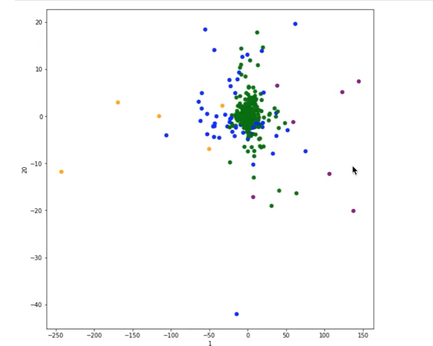
plt.figure(figsize=(10, 10))
# Create a list of four colors
colored = ['orange', 'green', 'blue', 'purple']
color = [colored[i] for i in predict]
plt.scatter(x[:, 1], x[:, 20], color=color)
plt.xlabel("1")
plt.ylabel("20")
plt.show()
print(silhouette_score(x, predict))Output results:
   order_id  product_id  ...  days_since_prior_order  aisle
0         2       33120  ...                     8.0   eggs
1        26       33120  ...                     7.0   eggs
2       120       33120  ...                    10.0   eggs
3       327       33120  ...                     8.0   eggs
4       390       33120  ...                     9.0   eggs
5       537       33120  ...                     3.0   eggs
6       582       33120  ...                    10.0   eggs
7       608       33120  ...                    12.0   eggs
8       623       33120  ...                     3.0   eggs
9       689       33120  ...                     3.0   eggs

[10 rows x 14 columns]
(206209, 27)
[1 1 1 1 1 1 1 1 1 1 1 1 1 1 1 1 1 1 1 1 1 1 1 1 1 1 3 1 1 1 1 1 1 1 1 1 0
 1 1 1 1 1 1 1 1 1 1 1 1 0 1 1 1 0 1 1 1 1 1 1 1 1 0 1 1 1 1 1 1 1 0 1 1 1
 0 1 1 1 1 1 1 1 1 1 1 0 1 1 0 1 1 1 1 1 1 1 1 1 1 1 1 1 1 1 1 1 1 1 1 0 1
 1 1 1 1 1 1 1 1 1 1 1 1 1 1 1 1 1 1 1 1 1 1 1 1 1 1 1 1 3 1 0 1 1 1 0 1 1
 1 1 1 3 0 1 1 1 1 1 1 1 0 1 1 1 1 1 1 1 1 1 1 1 0 1 1 1 1 1 1 0 1 1 1 1 1
 1 1 1 1 1 1 1 1 1 1 1 0 1 1 1 1 0 1 0 1 1 1 1 1 2 1 1 1 0 1 1 1 1 1 1 1 1
 3 1 1 1 0 1 1 1 1 0 0 0 1 0 1 1 1 1 1 1 0 1 1 1 1 0 1 1 1 1 1 1 1 1 1 1 1
 1 1 1 1 3 1 1 1 1 1 1 1 1 1 1 1 1 1 0 1 3 0 1 1 1 1 1 1 1 2 0 1 1 1 1 1 1
 1 1 1 1 1 1 1 1 1 1 1 1 0 1 1 1 2 1 1 1 1 1 1 1 0 1 3 1 1 1 3 1 1 1 1 1 1
 0 1 1 1 1 1 1 1 1 1 1 1 1 1 1 1 1 1 1 1 1 1 1 1 1 1 1 1 1 1 1 1 1 1 1 1 1
 1 1 2 1 1 1 1 1 1 1 0 1 1 1 1 1 1 1 1 0 1 1 1 1 1 1 1 0 1 1 1 1 0 1 1 1 1
 1 3 1 1 1 1 1 1 1 1 1 1 1 1 1 1 1 1 1 1 1 1 1 1 0 1 1 1 1 1 1 1 1 1 1 1 2
 1 1 1 0 1 1 1 0 1 0 1 1 1 1 1 1 1 3 1 0 0 0 1 1 1 1 1 1 1 1 1 1 1 1 1 1 0
 1 1 1 1 0 0 1 1 1 1 1 1 1 0 3 1 1 1 1]
Cluster scatter diagram:
15.K-means clustering effect evaluation criteria
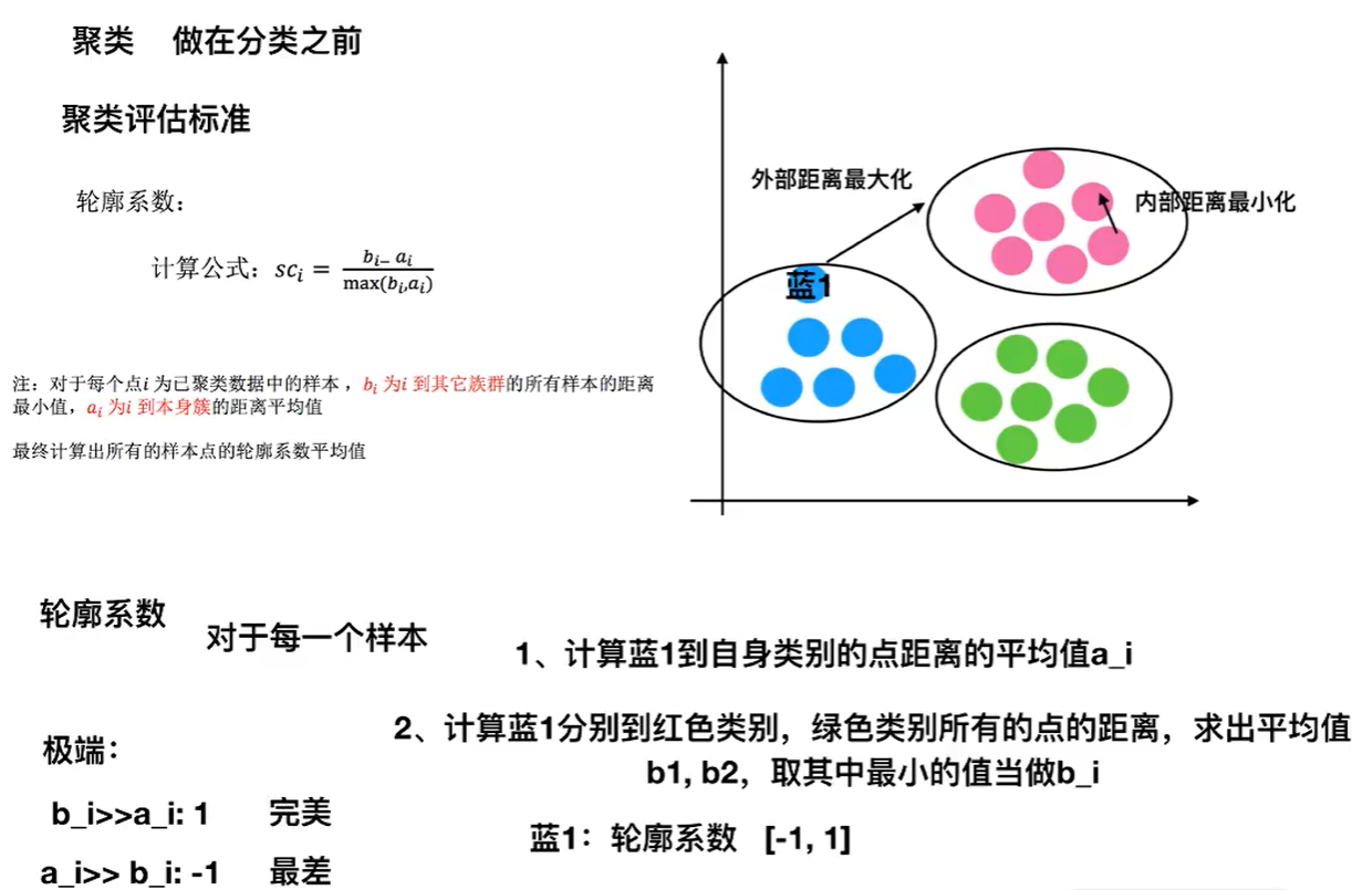
K-means--sklearn clustering effect evaluation API:
● sklearn.metrics.silhouette_score(X,labels)
● calculate the average contour coefficient of all samples
● X: characteristic value
● labels: target value (predicted value) marked by clustering
K-means summary:
Feature analysis: iterative algorithm is adopted, which is intuitive, easy to understand and very practical.
Disadvantages: it is easy to converge to the local optimal solution (multiple clustering)
Note: clustering is usually done before classification