introduction
As we all know, we brush questions before the exam. But most of the exams are not the original questions. What's the use of brushing questions before the exam? Of course, as like as two peas, we did not want to have the same questions in the exam. (maybe. In fact, in machine learning, the questions brushed before the test are the training set, the questions in the test are the new samples encountered after our model, and generalization is the performance of our model when encountering new samples (which corresponds to the score of the test).
Cross validation
After we train the model, we must want to see how the generalization of the model is. The general approach is to divide the data set into training set and test set. We use the training set to train the model and the test set to test the generalization ability of the model. We will also adjust the model according to the accuracy of the test set.

However, there is another problem, that is, if the model is adjusted according to the test set, the model is likely to be fitted on the test set, or if so, it will not reflect the generalization ability of the model.
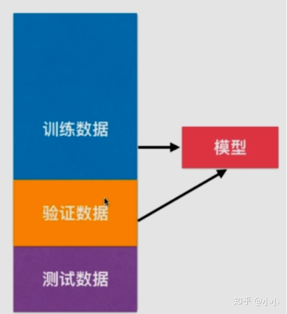
Therefore, more practice is to divide the data set into training set, verification set and test set. Through the training set training model, verify the set adjustment model, and test the generalization ability of the set test model.
However, the validation set also has randomness. It is likely that this validation set has over fitting, so cross validation occurs.

We randomly divide the training data into k parts, which is divided into k=3 parts in the figure above. Take any two combinations as the training set and the remaining group as the verification set, so as to obtain K models, and then take the mean value of K models as the result parameter. Obviously, this method is much more reliable than randomly using only one data set as the verification set.
Here is a practical example to see how to use cross validation parameters:
- The first case: use only the training set and the test set:
import numpy as np
from sklearn import datasets
from sklearn.model_selection import train_test_split
from sklearn.neighbors import KNeighborsClassifier

digits = datasets.load_digits()
x = digits.data
y = digits.target

x_train, x_test, y_train, y_test = train_test_split(x, y, test_size=0.4, random_state=666)

best_score, best_p, best_k = 0, 0, 0
for k in range(2, 11):
    for  p in range(1, 6):
        knn_clf = KNeighborsClassifier(weights="distance", n_neighbors=k, p=p)
        knn_clf.fit(x_train, y_train)
        score = knn_clf.score(x_test, y_test)
        if score > best_score:
            best_score, best_p, best_k = score, p, k

print("Best K=", best_k)
print("Best P=", best_p)
print("Best score=", best_score)
Output results
Best K= 3
Best P= 2
Best score= 0.9860917941585535
- The second case: use cross validation
from sklearn.model_selection import cross_val_score

knn_clf = KNeighborsClassifier()
cross_val_score(knn_clf, x_train, y_train)
# array([0.99537037, 0.98148148, 0.97685185, 0.97674419, 0.97209302])
According to the output results, by default, the cross validation of sklearn package is divided into 5 copies, which can also be modified through the cv parameter.
best_score, best_p, best_k = 0, 0, 0
for k in range(2, 11):
    for  p in range(1, 6):
        knn_clf = KNeighborsClassifier(weights="distance", n_neighbors=k, p=p)
        scores = cross_val_score(knn_clf, x_train, y_train)
        score = np.mean(scores)
        if score > best_score:
            best_score, best_p, best_k = score, p, k

print("Best K=", best_k)
print("Best P=", best_p)
print("Best score=", best_score)
Output results
Best K= 2
Best P= 2
Best score= 0.9851507321274763
It can be seen from the output results that the selected parameters are different from those before. Although the score has decreased by a point, it is more reliable to use cross validation. Of course, this is not the test score of the model.
best_knn_clf = KNeighborsClassifier(weights='distance', n_neighbors=2, p=2)
best_knn_clf.fit(x_train, y_train)
best_knn_clf.score(x_test, y_test)
The output result of 0.980528511821975 is the test score.
Bias variance tradeoff
Bias Variance Trade off, when our model performs poorly, there are usually two problems, one is high bias, the other is
High square difference problem. Identifying them helps to select the correct optimization method, so let's first look at the significance of deviation and variance.
- Deviation: describes the difference between the expected output result of the model and the real result of the sample.
- Variance: describes the output stability of the model for a given value. The greater the variance, the weaker the pan Chinese ability of the model.
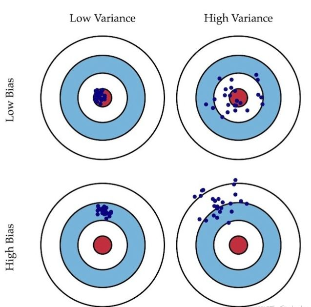
Just like shooting, deviation describes whether our overall shooting deviates from our goal, while variance describes the accuracy of shooting. The variance and deviation of the left one are very small, which are close to the center and concentrated. The right one is scattered near the center, but scattered, so the variance is large. In this way, it can be roughly understood by combining the following two figures. Deviation describes the gap between the expectation of the model output result and the real result of the sample. The variance describes the output stability of the model for a given value.
Model error = deviation + variance + unavoidable error
- The reason for the large deviation: the assumption of the problem itself is incorrect! For example, linear regression is used for nonlinear data. Or the height of the feature corresponding mark is irrelevant, which will also lead to high deviation. However, this corresponds to feature selection and has nothing to do with the algorithm. For the algorithm, it basically belongs to underfitting.
- Cause of large variance: a little disturbance of the data will greatly affect the model. The common reason is that the model used is too complex, such as high-order polynomial regression. This is called overfitting
- Summary: some algorithms are naturally high square difference algorithms, such as KNN. Nonparametric learning algorithms are usually high variance, because no assumptions are made on the data. Other algorithms are inherently highly biased, such as linear regression. Parameter learning is usually a high deviation algorithm because it has strong assumptions about data. Most algorithms have corresponding algorithms that can adjust the deviation and variance, such as k in KNN, such as degree in polynomial regression in linear regression. The deviation and variance are usually contradictory. Reducing the deviation will increase the variance, reducing the variance will increase the deviation, so it needs to be weighed in practical application. The main challenge of machine learning is variance. This sentence is only for algorithms, not for practical problems. Because most machine learning needs to solve the over fitting problem.
Solution: - Reduce model complexity
- Reduce data dimensions; noise reduction
- Increase the number of samples
- Use validation set
- Model regularization
Model regularization
Model Regularization: limit the size of parameters. It is often used to solve over fitting problems.
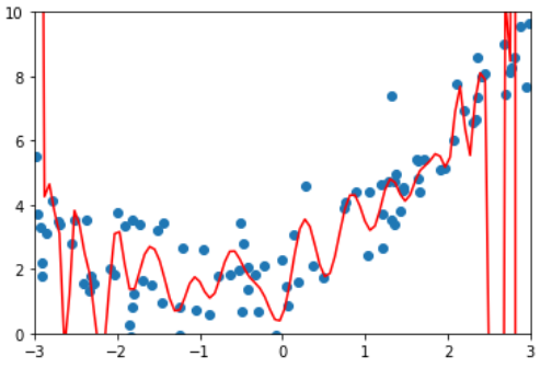
Let's first look at the polynomial regression over fitting:
from sklearn.linear_model import LinearRegression
from sklearn.pipeline import Pipeline
from sklearn.preprocessing import PolynomialFeatures
from sklearn.preprocessing import StandardScaler
from sklearn.metrics import mean_squared_error
import numpy as np
import matplotlib.pyplot as plt

def PolynomiaRegression(degree):
    return Pipeline([
        ('poly', PolynomialFeatures(degree=degree)),
        ('std_scale', StandardScaler()),
        ('lin_reg', LinearRegression()),
    ])

np.random.seed(666)
x = np.random.uniform(-3.0, 3.0, size=100)
X = x.reshape(-1, 1)
y = 0.5 * x**2 + x + 2 + np.random.normal(0, 1, size=100)

poly100_reg = PolynomiaRegression(degree=100)
poly100_reg.fit(X, y)
y100_predict = poly100_reg.predict(X)
mean_squared_error(y, y100_predict)
# 0.687293250556113
x_plot = np.linspace(-3, 3, 100).reshape(100, 1)
y_plot = poly100_reg.predict(x_plot)

plt.scatter(x, y)
plt.plot(x_plot[:,0], y_plot, color='r')
plt.axis([-3, 3, 0, 10])
plt.show()
lin_reg.coef_
array([ 1.21093453e+12,  1.19203091e+01,  1.78867645e+02, -2.95982349e+02,
       -1.79531458e+04, -1.54155027e+04,  8.34383276e+05,  8.19774042e+05,
       -2.23627851e+07, -1.44771550e+07,  3.87211418e+08,  1.13421075e+08,
       -4.61600312e+09, -1.25081501e+08,  3.93150405e+10, -5.47576783e+09,
       -2.44176251e+11,  5.46288687e+10,  1.11421043e+12, -2.76406464e+11,
       -3.71329259e+12,  8.55454910e+11,  8.80960804e+12, -1.60748867e+12,
       -1.39204160e+13,  1.49444708e+12,  1.19236879e+13,  2.47473079e+11,
        4.42409192e+11, -1.64280931e+12, -1.05153597e+13, -1.80898849e+11,
        3.00205050e+12,  2.75573418e+12,  8.74124346e+12, -1.36695399e+12,
       -1.22671920e+12, -7.00432918e+11, -8.24895441e+12, -8.66296096e+11,
       -2.75689092e+12,  1.39625207e+12,  6.26145077e+12, -3.47996080e+11,
        6.29123725e+12,  1.33768276e+12, -6.11902468e+11,  2.92339251e+11,
       -6.59758587e+12, -1.85663192e+12, -4.13408727e+12, -9.72012430e+11,
       -3.99030817e+11, -7.53702123e+11,  5.49214630e+12,  2.18518119e+12,
        5.24341931e+12,  7.50251523e+11,  5.50252585e+11,  1.70649474e+12,
       -2.26789998e+12, -1.84570078e+11, -5.47302714e+12, -2.86219945e+12,
       -3.88076411e+12, -1.19593780e+12,  1.16315909e+12, -1.41082803e+12,
        3.56349186e+12,  7.12308678e+11,  4.76397106e+12,  2.60002465e+12,
        1.84222952e+12,  3.06319895e+12, -1.33316498e+12,  6.18544545e+11,
       -2.64567691e+12, -1.01424838e+12, -4.76743525e+12, -3.59230293e+12,
       -1.68055178e+12, -3.57480827e+12,  2.06629318e+12, -6.07564696e+11,
        3.40446395e+12,  3.42181387e+12,  3.31399498e+12,  4.92290870e+12,
        3.79985951e+11,  1.34189037e+12, -3.34878352e+12, -2.07865615e+12,
       -3.24634078e+12, -5.48903768e+12,  5.87242630e+11, -2.27318874e+12,
        2.60023097e+12,  8.21820883e+12,  4.79532121e+10, -3.11436610e+12,
       -6.27736909e+11])
By looking at the coefficients of polynomial regression, it can be found that some coefficients can be 13 orders of magnitude worse. In fact, this is over fitting! Model regularization is to solve this problem. Let's first review the objectives of polynomial regression.
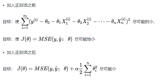
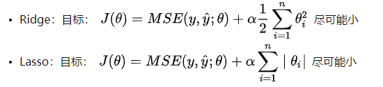
By adding the regular term to control the coefficient not to be too large, so that the curve is not so steep and changes so violently. Here are a few details to note.
- First point: θ Starting from 1, only the coefficient is included, not the intercept, because the intercept only determines the height of the curve and does not affect the steepness and ease of the curve.
- Point 2: this 1 / 2 is to eliminate 2 after derivation, so as to facilitate calculation. But in fact, whether this is possible or not, because there is a coefficient before regularization, and we can take this 1 / 2 into account ɑ Go.
- Point 3: coefficient ɑ, It represents the proportion of regularization term in the whole loss function. At the extreme, ɑ= 0, it is equivalent that the model does not add regularization, but if ɑ= It is infinite. At this time, the main optimization task becomes the need for all ɑ Are as small as possible, and the optimal case is all 0. as for ɑ You need to try.
Ridge regression

Test case:
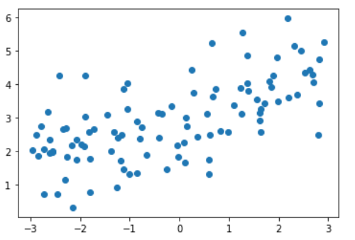
import numpy as np
import matplotlib.pyplot as plt

np.random.seed(42)
x = np.random.uniform(-3.0, 3.0, size=100)
X = x.reshape(-1, 1)
y = 0.5 * x + 3 + np.random.normal(0, 1, size=100)

plt.scatter(x, y)
plt.show()
from sklearn.linear_model import LinearRegression
from sklearn.pipeline import Pipeline
from sklearn.preprocessing import PolynomialFeatures
from sklearn.preprocessing import StandardScaler
from sklearn.model_selection import train_test_split
from sklearn.metrics import mean_squared_error
def PolynomiaRegression(degree):
return Pipeline([
('poly', PolynomialFeatures(degree=degree)),
('std_scale', StandardScaler()),
('lin_reg', LinearRegression()),
])
np.random.seed(666)
x_train, x_test, y_train, y_test = train_test_split(X, y)
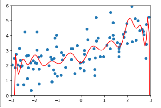
poly_reg = PolynomiaRegression(degree=20)
poly_reg.fit(x_train, y_train)
y_poly_predict = poly_reg.predict(x_test)
mean_squared_error(y_test, y_poly_predict)
# 167.9401085999025
import matplotlib.pyplot as plt
x_plot = np.linspace(-3, 3, 100).reshape(100, 1)
y_plot = poly_reg.predict(x_plot)
plt.scatter(x, y)
plt.plot(x_plot[:,0], y_plot, color='r')
plt.axis([-3, 3, 0, 6])
plt.show()
Encapsulate the drawing operations into a function for later calls:
def plot_model(model):
    x_plot = np.linspace(-3, 3, 100).reshape(100, 1)
    y_plot = model.predict(x_plot)

    plt.scatter(x, y)
    plt.plot(x_plot[:,0], y_plot, color='r')
    plt.axis([-3, 3, 0, 6])
    plt.show()
Using ridge regression:
from sklearn.linear_model import Ridge
def RidgeRegression(degree, alpha):
return Pipeline([
('poly', PolynomialFeatures(degree=degree)),
('std_scale', StandardScaler()),
('lin_reg', Ridge(alpha=alpha)),
])
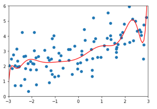
ridege1_reg = RidgeRegression(20, alpha=0.0001)
ridege1_reg.fit(x_train, y_train)
y1_predict = ridege1_reg.predict(x_test)
mean_squared_error(y_test, y1_predict)
# 1.3233492754136291
# It is much smaller than the previous 136
plot_model(ridege1_reg)

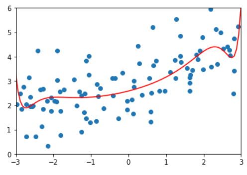
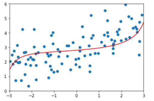
ridege2_reg = RidgeRegression(20, alpha=1)
ridege2_reg.fit(x_train, y_train)

y2_predict = ridege2_reg.predict(x_test)
mean_squared_error(y_test, y2_predict)
# 1.1888759304218461
plot_model(ridege2_reg)
ridege3_reg = RidgeRegression(20, alpha=100)
ridege3_reg.fit(x_train, y_train)

y3_predict = ridege3_reg.predict(x_test)
mean_squared_error(y_test, y3_predict)
# 1.3196456113086197
# At this time, compared with alpha=1, the mean square error increases, indicating that it may be excessive
plot_model(ridege3_reg)
ridege4_reg = RidgeRegression(20, alpha=1000000)
ridege4_reg.fit(x_train, y_train)

y4_predict = ridege4_reg.predict(x_test)
mean_squared_error(y_test, y4_predict)
# 1.8404103153255003
plot_model(ridege4_reg)
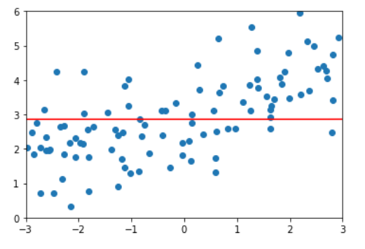
This is also the same as the previous analysis, if ɑ= At positive infinity, in order to minimize the loss function, it is necessary to minimize the sum of squares of all coefficients, that is θ All tend to 0. It can be seen from the above alpha values that we can search more carefully in 1-100 to find the most suitable relatively smooth curve to fit. This is L2 regularity.
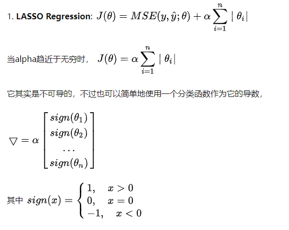
LASSO Regularization

LASSO: Least Absolute Shrinkage and Selection Operator Regression
Shrink: shrink, shrink, shrink. Feature reduction. The focus is on the Selection Operator
Using lasso regression:
from sklearn.linear_model import Lasso

def LassoRegression(degree, alpha):
    return Pipeline([
        ('poly', PolynomialFeatures(degree=degree)),
        ('std_scale', StandardScaler()),
        ('lin_reg', Lasso(alpha=alpha)),
    ])

lasso1_reg = LassoRegression(20, 0.01)
#This is much smaller than Ridge's alpha because it is the square term in Ridge
lasso1_reg.fit(x_train, y_train)

y1_predict = lasso1_reg.predict(x_test)
mean_squared_error(y_test, y1_predict)
# 1.149608084325997
plot_model(lasso1_reg)
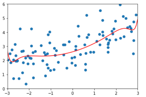
lasso2_reg = LassoRegression(20, 0.1)
lasso2_reg.fit(x_train, y_train)

y2_predict = lasso2_reg.predict(x_test)
mean_squared_error(y_test, y2_predict)
# 1.1213911351818648
plot_model(lasso2_reg)

lasso3_reg = LassoRegression(20, 1)
lasso3_reg.fit(x_train, y_train)

y3_predict = lasso3_reg.predict(x_test)
mean_squared_error(y_test, y3_predict)
# 1.8408939659515595
plot_model(lasso3_reg)
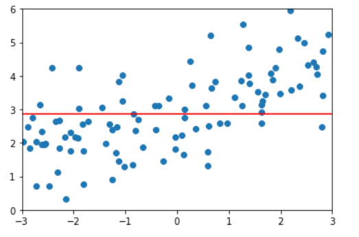
Explain Ridge and LASSO
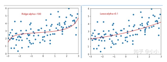
By comparing the two figures, it is found that the model fitted by Lasso tends to be a straight line, while the model fitted by ridge tends to be a curve. This is because the essence of two regularities is different. Ridge tends to make all θ The sum of is as small as possible, while Lasso tends to make a part θ The value of becomes 0, so it can be used as feature selection, which is why it is called Selection Operation.
Let's try to explain the above two sentences:
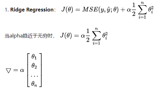
In derivative θ All have values and fall along the gradient. Ridge tends to make all θ The sum of is as small as possible, rather than being directly 0 as lasso.
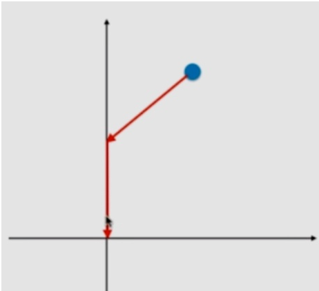
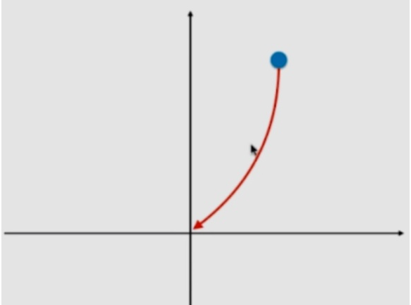
Therefore, if the gradient descent starts from a point in the figure above, you can't approach 0 curvilinearly like Ridge, but can only use these very regular ways to approach the zero point. In the gradient descent of this path, the zero point of some axes will be reached, and lasso tends to make part of it θ The value of becomes 0. So it can be used as feature selection. However, it is precisely because of such characteristics that lasso may mistakenly change the coefficient of the original useful features to 0. Therefore, compared with Ridge, Ridge has a better accuracy. However, when the features are particularly large, Lasso can also reduce the features of the model.
Elastic net
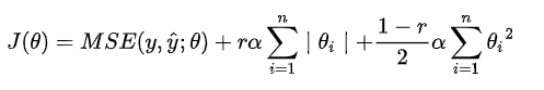
Since the two have their own advantages, we should combine them, which is Elastic Net.