linear regression

Understanding of Regression

Nature allows us to return to a certain range; conversely, there is an average level that allows prominent things to move closer to him.
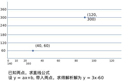
Begin with what we know best. linear equation

General steps of linear regression

loss function

Loss (Cost) Function Introduction
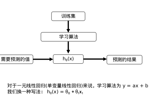
What linear regression actually needs to do is to select the appropriate parameters (w, b), so that the f(x) equation can fit the training set well.
Model: h theta(x) = theta 0+theta 1x1
Parameters: Theta 0, Theta 1
Loss function:

Objective: To minimize the loss function. j (theta 0, theta 1)

gradient descent

I. Gradient Method Thought
The three elements of gradient method are starting point, descending direction and descending step.
The objective function of machine learning is usually convex function. What is convex function? Limited to space, we do not do very deep expansion. Here we make an image metaphor, convex function to solve the problem, we can imagine the objective loss function as a pot to find the bottom of the pot. The very intuitive idea is that we go down the gradient direction of the function at the initial point (that is, the gradient descent). Here, we make another image analogy. If we compare this walking method with force, then the complete three elements are step length, direction and starting point. This image analogy makes our solution to the gradient problem clear and clear. The starting point is very important. It is the key point to consider when initializing, while direction and starting point. Step size is the key. In fact, the difference between different gradients lies in the difference between these two points.
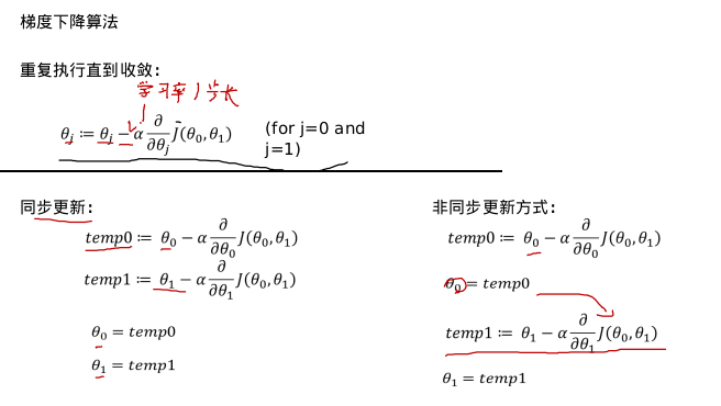
Direction of gradient descent 1: As long as the loss function is derived, the variation direction of theta always approaches the minimum value of the loss function.
Direction of descent of gradient 2: If theta is already at the lowest point, the gradient will not change.
Whether the slope is positive or negative, the gradient decreases gradually to the minimum. If alpha is too small, the gradient decreases very slowly. If alpha is too large, the gradient descent over the minimum value will not converge, but may diverge.
The gradient of linear regression decreases.

Batch Gradient Descent Batch Gradient Descent Batch Gradient Descent Batch Gradient Descent: Batch Gradient Descent: Batch Gradient Descent Batch Gradient Descent is calculated using all training sets for each step of descent. Therefore, each update will proceed in the right direction. Finally, it can ensure convergence to extreme point, convex function to global extreme point, non-convex function may converge to local extreme point. The drawback is that the learning time is too long and a large amount of memory is consumed.
Stochastic Gradient Descent Random Gradient Decline: Random Gradient Decline: A training set is used to calculate the gradient value for each step of descent.
The disadvantage of SGD is that each update may not be carried out in the right direction. The parameter update has high variance, which leads to sharp fluctuation of loss function. However, if the objective function has basin region, SGD will make the optimization direction jump from the current local minimum point to another better local minimum point, so that for non-convex functions, it may eventually converge to a better local extreme point, or even a global extreme point.
Take a simple example.

"""
//Random gradient descent
"""
import numpy as np
import random
X = 2 * np.random.rand(100, 1)
y = 4 + 3 * X + np.random.randn(100, 1)
X_b = np.c_[np.ones((100, 1)), X]

n_epochs = 500
a0 = 0.1
decay_rate = 1

m = 100
num = [i for i in range(100)]

def learning_schedule(epoch_num):
    return (1 / (decay_rate * epoch_num + 1)) * a0
theta = np.random.randn(2, 1)

# epoch means round, which means doing an iteration with m samples
for epoch in range(n_epochs):
    # Generate 100 unrepeated random numbers
    rand = random.sample(num, 100)
    for i in range(m):
        random_index = rand[i]
        xi = X_b[random_index:random_index+1]
        yi = y[random_index:random_index+1]
        gradients = xi.T.dot(xi.dot(theta)-yi)
        learning_rate = learning_schedule(epoch+1)
        theta = theta - learning_rate * gradients
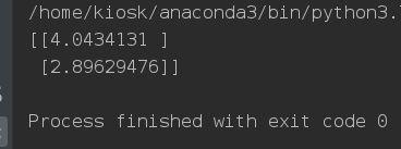
print(theta)

"Mini-Batch" Gradient Descent "Mini-Batch" gradient descent: "Mini-Batch" gradient descent: refers to the use of a part of the training set to calculate the gradient value for each step of descent. SGD converges faster than BGD, however, it also has the disadvantage of floating and unstable when convergence, fluctuating near the optimal solution, and it is difficult to judge whether it has converged. At this time, the compromise algorithm of small batch gradient descent method, MBGD came into being, the reason is simple, SGD is too extreme, one at a time, why not more than a few? MBGD is a method of iterating multiple data at a time. We are also just an example.

import numpy as np
import random

X = 2 * np.random.rand(100, 1)
y = 4 + 3 * X + np.random.randn(100, 1)
X_b = np.c_[np.ones((100, 1)), X]

n_epochs = 500
t0, t1 = 5, 50

m = 100
num = [i for i in range(100)]

def learning_schedule(t):
    return t0 / (t + t1)

theta = np.random.randn(2, 1)
batch_num = 5
batch_size = m // 5

for epoch in range(n_epochs):
    # Generate 100 unrepeated random numbers
    for i in range(batch_num):
        start = i*batch_size
        end = (i+1)*batch_size
        xi = X_b[start:end]
        yi = y[start:end]
        gradients = 1/batch_size * xi.T.dot(xi.dot(theta)-yi)
        learning_rate = learning_schedule(epoch*m + i)
        theta = theta - learning_rate * gradients
print(theta)