This blog article will summarize the use of pytorch, a deep learning framework.
Explanation of Tensors
Scalar is a quantity with only size and no direction, such as 1, 2, 3, etc.
Vector is a quantity with size and direction, which is actually a series of numbers, such as (1,2)
Matrix is a bunch of numbers, such as [1,2;3,4], which are composed of several vectors in a row.
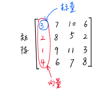
Scalar, vector and matrix are also tensors. Scalar is a zero-dimensional tensor, vector is a one-dimensional tensor, and matrix is a two-dimensional tensor.

In addition, tensors can be four-dimensional, five-dimensional and so on.
Code example:
import torch
x=torch.Tensor(2,3)##Two-dimensional tensor
print x

1.0860e+32  4.5848e-41  7.0424e-38
0.0000e+00  4.4842e-44  0.0000e+00
[torch.FloatTensor of size 2x3]
import torch
x=torch.Tensor(4,2,3)##Three-dimensional tensor
print x
(0 ,.,.) =
-7.7057e-06 4.5772e-41 -7.7057e-06
4.5772e-41 0.0000e+00 0.0000e+00
(1 ,.,.) =
0.0000e+00 0.0000e+00 0.0000e+00
0.0000e+00 8.1459e-38 0.0000e+00
(2 ,.,.) =
nan 0.0000e+00 7.7143e-28
2.5353e+30 1.8460e+31 1.7466e+19
(3 ,.,.) =
1.8430e-37 0.0000e+00 nan
nan 6.0185e-36 2.4062e-38
[torch.FloatTensor of size 4x2x3]The tensor y of 4x2x3 consists of four 2x3 matrices.
Conversion between torch.tensor and numpy.array
import torch
import numpy as np

np_data = np.arange(6).reshape((2, 3))
torch_data = torch.from_numpy(np_data)##Convert numpy.array to torch.tensor
tensor2array = torch_data.numpy()##Convert torch.tensort to numpy.array

print torch_data
print tensor2array,type(tensor2array)

 0  1  2
 3  4  5
[torch.LongTensor of size 2x3]

[[0 1 2]
[3 4 5]]
<type 'numpy.ndarray'>
Some Mathematical Operations in Pyrtorch
# Absolute value calculation of abs
data = [-1, -2, 1, 2]
tensor = torch.FloatTensor(data)  # Converting to 32-bit floating-point tensor
print(
    '\nabs',
    '\nnumpy: ', np.abs(data),          # [1 2 1 2]
    '\ntorch: ', torch.abs(tensor)      # [1 2 1 2]
)

# Sin trigonometric function sin
print(
    '\nsin',
    '\nnumpy: ', np.sin(data),      # [-0.84147098 -0.90929743  0.84147098  0.90929743]
    '\ntorch: ', torch.sin(tensor)  # [-0.8415 -0.9093  0.8415  0.9093]
)

# Mean mean value
print(
    '\nmean',
    '\nnumpy: ', np.mean(data),         # 0.0
    '\ntorch: ', torch.mean(tensor)     # 0.0
)
Matrix operations:
# matrix multiplication matrix point multiplication
data = [[1,2], [3,4]]
tensor = torch.FloatTensor(data)  # convert to32Bit floating point tensor
# correct method
print(
    '\nmatrix multiplication (matmul)',
    '\nnumpy: ', np.matmul(data, data),     # [[7, 10], [15, 22]]
    '\ntorch: ', torch.mm(tensor, tensor)   # [[7, 10], [15, 22]]
)

# !!!!!! The following is the wrong way!!!!
data = np.array(data)
print(
    '\nmatrix multiplication (dot)',
    '\nnumpy: ', data.dot(data),        # [[7, 10], [15, 22]] stay numpy Feasible in
    '\ntorch: ', tensor.dot(tensor)     # torch converts to [1,2,3,4].dot([1,2,3,4) = 30.0
)
Matrix addition:
import torch
import numpy as np

a=torch.rand(5,3)
b=torch.rand(5,3)

print "a",a
print "b",b

print "a+b",a+b
print "torch.add(a,b)",torch.add(a,b)

res=torch.Tensor(5,3)

print "torch.add(a,b,out=res)",torch.add(a,b,out=res)##Store the result of the operation on res

print "b.add_(a)",b.add_(a)##Result Coverage b

a
 0.0540  0.2670  0.6704
 0.7695  0.9178  0.8770
 0.6552  0.4423  0.1735
 0.1376  0.1208  0.6674
 0.7257  0.1426  0.1134
[torch.FloatTensor of size 5x3]

b
 0.4811  0.7744  0.7762
 0.5247  0.6045  0.6148
 0.8366  0.8996  0.5378
 0.5236  0.4987  0.9592
 0.8462  0.8286  0.5010
[torch.FloatTensor of size 5x3]

a+b
 0.5350  1.0413  1.4466
 1.2942  1.5223  1.4918
 1.4918  1.3419  0.7113
 0.6612  0.6195  1.6266
 1.5719  0.9712  0.6144
[torch.FloatTensor of size 5x3]

torch.add(a,b)
 0.5350  1.0413  1.4466
 1.2942  1.5223  1.4918
 1.4918  1.3419  0.7113
 0.6612  0.6195  1.6266
 1.5719  0.9712  0.6144
[torch.FloatTensor of size 5x3]

torch.add(a,b,out=res)
 0.5350  1.0413  1.4466
 1.2942  1.5223  1.4918
 1.4918  1.3419  0.7113
 0.6612  0.6195  1.6266
 1.5719  0.9712  0.6144
[torch.FloatTensor of size 5x3]

b.add_(a)
 0.5350  1.0413  1.4466
 1.2942  1.5223  1.4918
 1.4918  1.3419  0.7113
 0.6612  0.6195  1.6266
 1.5719  0.9712  0.6144
[torch.FloatTensor of size 5x3]
Tensor's partial interception is very similar to the slice in numpy, and the operation is almost the same.
autograd automatic differential
Variable:
If we understand each tensor Tensor as an egg, then Variable is the basket in which these eggs are stored (torch.Tensor).
import torch
from torch.autograd import Variable # Variable module in torch

# Mr. eggs
tensor = torch.FloatTensor([[1,2],[3,4]])
# Put the eggs in the basket. Require_grad does not participate in the back propagation of errors. Do you need to calculate the gradient?
variable = Variable(tensor, requires_grad=True)

print(tensor)
"""
 1  2
 3  4
[torch.FloatTensor of size 2x2]
"""

print(variable)
"""
Variable containing:
 1  2
 3  4
[torch.FloatTensor of size 2x2]
Variable calculation, gradient
Variable is used to wrap tensor and replace wrapped tensor with Variable to perform a series of operations. It silently builds a huge system behind the background screen step by step, called computational graph. What is this graph used for? It used to connect all calculation steps (nodes) together, and finally, when the error is transmitted backward, it will be used once. The magnitude of modification (gradient) in variable is calculated.
import torch
import numpy as np
from torch.autograd import Variable

x=Variable(torch.ones(2),requires_grad=True)##Cover a tensor (2*1) with Variable, and set require_grad=True to participate in error back propagation, to calculate the gradient

z=4*x*x
y=z.norm()

print "y:",y

y.backward()## Backward calculation
print "x.grad:",x.grad##Calculate the gradient of y to X

//Printout
y: Variable containing:
 5.6569
[torch.FloatTensor of size 1]

x.grad: Variable containing:
 5.6569
 5.6569
[torch.FloatTensor of size 2]
It should be noted that autograd is specially designed for BP algorithm, so this autograd is only useful for scalar output value, because the output of loss function is a scalar. If y is a vector, the backward() function will fail.
The internal mechanism of autograd:
Autograd can be achieved thanks to Variable and Function data types. To do autograd, you must first convert tensor data into Variable. Varibale and tensor are basically the same, except for the following attributes.
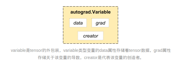
The data attribute returns the original tensor value wrapped in the Variable, which converts a Variable type into a tensor type; the grad attribute returns its gradient value.
variable and function are inseparable from each other:
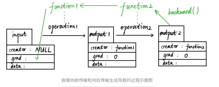
As shown in the figure, suppose that we have an input variable input (data type is Variable) which is input by the user, so its creator is null value. Input obtains output 1 variable (data type is still Variable) through the first data operation operation1 (such as addition, subtraction, multiplication and division), which automatically generates a Function 1 variable (data type is Functional). An example) and the creator of output 1 is this Function 1. Subsequently, output 1 generates output 2 through another data operation, which also generates another instance, Function 2, whose creator is Function 2.
In this forward propagation process, function 1 and function 2 record all the operation history of data input. When output 2 runs its backward function, function 2 and function 1 automatically reverse-compute the derivative value of input and store it in the grad attribute.
A variable whose creator is null can be returned to a derivative, such as input. If the entire operation flow is considered as a graph (Graph), then a creator such as input is called a graph leaf. Creator variables that are not null, such as output1 and output2, cannot be returned as derivatives, and their grads are all zero. So only leaf nodes can be autograd ed.
Get the data in Variable
print(variable)     #  Variable form
"""
Variable containing:
 1  2
 3  4
[torch.FloatTensor of size 2x2]
"""

print(variable.data)    # tensor form
"""
 1  2
 3  4
[torch.FloatTensor of size 2x2]
"""

print(variable.data.numpy())    # numpy form
"""
[[ 1.  2.]
 [ 3.  4.]]
Incentive function
import torch
import torch.nn.functional as F     # The excitation functions are all here.
from torch.autograd import Variable

# Do some fake data to watch the image
x = torch.linspace(-5, 5, 200)  # x data (tensor), shape=(100, 1)
x = Variable(x)


x_np = x.data.numpy()   # Change to numpy array for drawing

# Several commonly used excitation functions
y_relu = F.relu(x).data.numpy()
y_sigmoid = F.sigmoid(x).data.numpy()
y_tanh = F.tanh(x).data.numpy()
y_softplus = F.softplus(x).data.numpy()
# Y_softmax = F. softmax (x) softmax is special and cannot be displayed directly, but it is about probability and is used for classification.
pytorch for regression fitting
Create some false data to simulate the real situation. For example, a quadratic function of one variable: y = a * x^2 + b. Let's add a little noise to the Y data to show it more authentically.
#coding:utf-8
import torch
from torch.autograd import Variable
import matplotlib.pyplot as plt
import torch.nn.functional as F

x=torch.unsqueeze(torch.linspace(-1,1,100),dim=1)##torch.unsqueeze returns a new tensor and adds a new dimension at position 1, returning a tensor with a shape of (100,1)
y=x.pow(2)+0.2*torch.rand(x.size()) ##Add a little noise to y
x,y=Variable(x),Variable(y) ##Using Variabvle to wrap tensor is convenient for later gradient calculation, and the neural network can only accept Variable type data.


class Net(torch.nn.Module):
    def __init__(self,n_feature,n_hidden,n_output):##Customize various layers
        super(Net,self).__init__()
        self.hidden=torch.nn.Linear(n_feature,n_hidden)
        self.predict=torch.nn.Linear(n_hidden,n_output)

    def forward(self, x): ##Build a Neural Network
        x=F.relu(self.hidden(x)) ##x arrives at hiddenlayer and is activated by relu
        x=self.predict(x)##When x reaches the output layer, the output layer does not need to be activated, because there is no interval limit on the size of the predicted value in the regression problem, and if the activation layer is used, a part of it will be truncated.
        return x

net=Net(n_feature=1,n_hidden=10,n_output=1)
print net

optimizer=torch.optim.Adam(net.parameters(),lr=0.2) # All parameters passed into net, learning rate
loss_func=torch.nn.MSELoss()# The Error Formula of Predictive Value and Real Value (Mean Variance)

plt.ion()
plt.show()
for t in range(100):
    prediction=net(x)# Feed net training data x, output predictive value

    loss=loss_func(prediction,y)  # Calculating the Errors of the Two

    optimizer.zero_grad()# Clean up the residual parameter gradient of the last reverse update of all parameters, because the gradient of each parameter will be retained every time the parameters are updated in reverse (BP algorithm).
    loss.backward()  ##Calculate the gradient of each parameter according to the error
    optimizer.step()   # Update parameters with learning efficiency lr=0.2, w=w-lr*alpha(loss)/alpha(w)


    if t%5 == 0:
        plt.cla()##In dynamic drawing, each time a new drawing is drawn, the drawing drawn at the previous moment is erased.
        plt.scatter(x.data.numpy(),y.data.numpy())
        plt.plot(x.data.numpy(),prediction.data.numpy(),'r-',lw=5)
        plt.pause(0.5)