Machine learning experiment 2: support vector machine

Keywords: Python Machine Learning sklearn

introduce

In this experiment, we will use support vector machine (SVM) and understand its working principle on data.

The data sets used in this experiment include:

ex2data1.mat - linear SVM classification dataset
ex2data2.mat - Gaussian kernel SVM classification dataset
ex2data3.mat - cross validation Gaussian kernel SVM classification dataset

The scoring criteria are as follows:

Point 1: use linear SVM -----------------(20 points)
Point 2: define Gaussian kernel ---------------------(20 points)
Point 3: use Gaussian kernel SVM ---------------(20 points)
Key point 4: search for the optimal parameters of SVM ------------(20 points)
Point 5: handwritten numeral recognition ---------------(20 points)

In [120]:

# Import the required library files
import numpy as np
import pandas as pd
import matplotlib.pyplot as plt
from scipy.io import loadmat
import os

%matplotlib inline

1 linear SVM

In this part of the experiment, linear SVM classification will be realized and applied to data set 1.

In [121]:

raw_data = loadmat('ex2data1.mat')
data = pd.DataFrame(raw_data.get('X'), columns=['X1', 'X2'])
data['y'] = raw_data.get('y')

data.head()

Out[121]:

	X1	X2	y
0	1.9643	4.5957	1
1	2.2753	3.8589	1
2	2.9781	4.5651	1
3	2.9320	3.5519	1
4	3.5772	2.8560	1

In [122]:

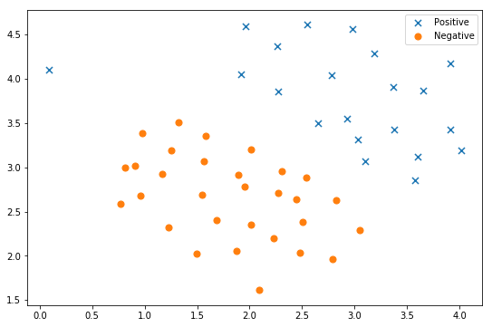
# Define data visualization functions 
def plot_init_data(data, fig, ax):
    positive = data[data['y'].isin([1])]
    negative = data[data['y'].isin([0])]

    ax.scatter(positive['X1'], positive['X2'], s=50, marker='x', label='Positive')
    ax.scatter(negative['X1'], negative['X2'], s=50, marker='o', label='Negative')

In [123]:

# Data visualization
fig, ax = plt.subplots(figsize=(9,6))
plot_init_data(data, fig, ax)
ax.legend()
plt.show()

**Important point 1: * * the * * task in this part is to apply linear SVM to dataset 1: ` ex2data1.mat '** You can call the sklearn library to realize the SVM function.

In [124]:

from sklearn import svm
# ======================Fill in the code here======================= 
svc = svm.SVC(kernel="linear")
svc.fit(data[['X1', 'X2']], data['y'])
svc.score(data[['X1', 'X2']], data['y'])
# =============================================================

Out[124]:

0.9803921568627451

In [125]:

#Define visual classification boundary functions
def find_decision_boundary(svc, x1min, x1max, x2min, x2max, diff):
    x1 = np.linspace(x1min, x1max, 1000)
    x2 = np.linspace(x2min, x2max, 1000)

    cordinates = [(x, y) for x in x1 for y in x2]
    x_cord, y_cord = zip(*cordinates)
    c_val = pd.DataFrame({'x1':x_cord, 'x2':y_cord})
    c_val['cval'] = svc.decision_function(c_val[['x1', 'x2']])

    decision = c_val[np.abs(c_val['cval']) < diff]
    
    return decision.x1, decision.x2

In [126]:

#Display classification decision surface
x1, x2 = find_decision_boundary(svc, 0, 4, 1.5, 5, 2 * 10**-3)
fig, ax = plt.subplots(figsize=(9,6))
ax.scatter(x1, x2, s=10, c='r',label='Boundary')
plot_init_data(data, fig, ax)
ax.set_title('SVM (C=1) Decision Boundary')
ax.legend()
plt.show()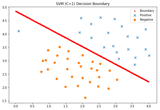

In [127]:

#Try C=100
svc2 = svm.LinearSVC(C=100, loss='hinge', max_iter=1000)
svc2.fit(data[['X1', 'X2']], data['y'])
svc2.score(data[['X1', 'X2']], data['y'])

/opt/conda/lib/python3.6/site-packages/sklearn/svm/base.py:931: ConvergenceWarning: Liblinear failed to converge, increase the number of iterations.
  "the number of iterations.", ConvergenceWarning)

Out[127]:

0.9411764705882353

In [128]:

#Display classification decision surface
x1, x2 = find_decision_boundary(svc2, 0, 4, 1.5, 5, 2 * 10**-3)
fig, ax = plt.subplots(figsize=(9,6))
ax.scatter(x1, x2, s=10, c='r',label='Boundary')
plot_init_data(data, fig, ax)
ax.set_title('SVM (C=100) Decision Boundary')
ax.legend()
plt.show()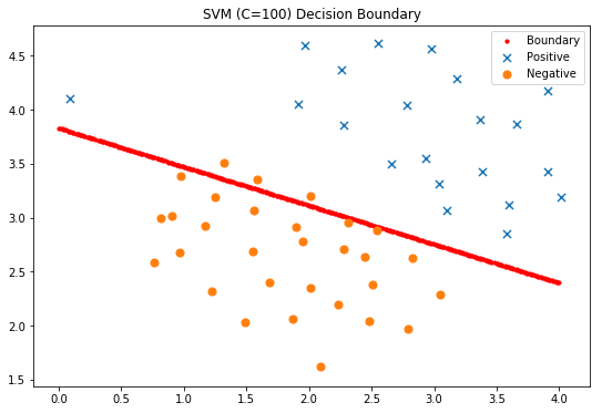

2 Gaussian kernel SVM

In this part of the experiment, the kernel SVM will be used to realize the nonlinear classification task.

2.1 Gaussian kernel

For two samples x1,x2 ∈ Rdx1,x2 ∈ Rd, the Gaussian kernel is defined as

Kgaussian(x1,x2)=exp(−∥x1−x2∥222σ2)Kgaussian(x1,x2)=exp⁡(−‖x1−x2‖222σ2)

**Key point 2: * * the * * task of this part is to realize the definition of Gaussian kernel function according to the above formula**

In [129]:

def gaussianKernel(x1, x2, sigma):
    """
    Define Gaussian kernel.
    
    input parameter 
    ----------
    x1 :  First sample point, size(d,1)Vector of
    
    x2 :  The second sample point, the size is(d,1)Vector of
    
    sigma : Bandwidth parameters of Gaussian kernel

    Output results
    -------
    sim : Similarity of two samples (similarity). 
    
    """
# ======================Fill in the code here======================= 
    sim=np.exp(-np.power(x1-x2, 2).sum()/(2*sigma**2))

# ============================================================= 
    return sim

If the above Gaussian kernel function is completed Gaussian kernel, the following code can be used for testing. If the result is 0.324652, the calculation passes.

In [130]:

#Test Gaussian kernel function
x1 = np.array([1, 2, 1])
x2 = np.array([0, 4, -1])
sigma = 2

sim = gaussianKernel(x1, x2, sigma)

print('Gaussian Kernel between x1  and x2 is :', sim)

Gaussian Kernel between x1  and x2 is : 0.32465246735834974

2.2 Gaussian kernel SVM applied to dataset 2

In this experiment, Gaussian kernel SVM is applied to data set 2: ex2data2.mat..

In [131]:

raw_data = loadmat('ex2data2.mat')

data = pd.DataFrame(raw_data['X'], columns=['X1', 'X2'])
data['y'] = raw_data['y']

fig, ax = plt.subplots(figsize=(9,6))
plot_init_data(data, fig, ax)
ax.legend()
plt.show()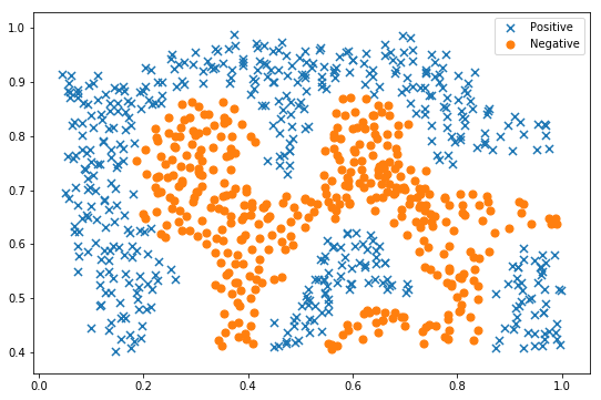

As can be seen from the above figure, the above two types of samples are linearly inseparable. Kernel SVM is needed for classification.

**Point 3: * * the * * task of this part is to apply Gaussian kernel SVM to dataset 2** The sklearn library can be called to realize the nonlinear SVM function.

In [132]:

# ======================Fill in the code here======================= 
svc = svm.SVC( kernel='rbf', gamma=30)
svc.fit(data[['X1', 'X2']], data['y'])
svc.score(data[['X1', 'X2']], data['y'])

# =============================================================

Out[132]:

0.9721900347624566

In [133]:

x1, x2 = find_decision_boundary(svc, 0, 1, 0.4, 1, 0.01)
fig, ax = plt.subplots(figsize=(9,6))
plot_init_data(data, fig, ax)
ax.scatter(x1, x2, s=10)
plt.show()

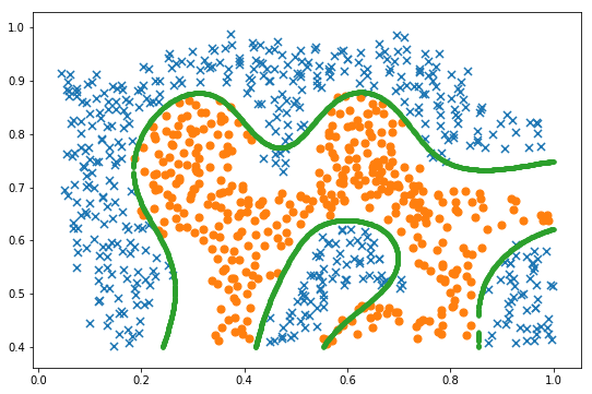
3 cross validation Gaussian kernel SVM

In this part of the experiment, the optimal parameters CC and CC of Gaussian kernel SVM will be selected by cross validation method σσ， And apply it to dataset 3: ex2data3.mat. The data set contains training sample set X (training sample characteristics), y (training sample marker) and validation set Xval (validation sample characteristics), yval (validation sample mark).

In [134]:

raw_data = loadmat('ex2data3.mat')

X = raw_data['X']
Xval = raw_data['Xval']
y = raw_data['y'].ravel()
yval = raw_data['yval'].ravel()

fig, ax = plt.subplots(figsize=(9,6))
data = pd.DataFrame(raw_data.get('X'), columns=['X1', 'X2'])
data['y'] = raw_data.get('y')
plot_init_data(data, fig, ax)
plt.show()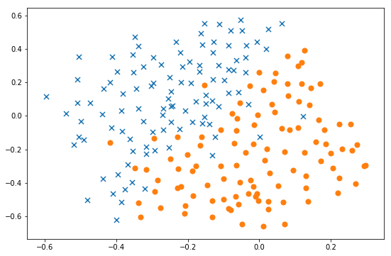

3.1 search SVM optimal parameters CC and σσ

**Key point 4: * * the * * task of this part is to search the optimal parameters CC and CC of SVM σσ. ** For CC and σσ， You can search from the following candidate sets {0.01,0.03,0.1,0.3,1,3,10,30}{0.01,0.03,0.1,0.3,1,3,10,30}

In [135]:

C_values = [0.01, 0.03, 0.1, 0.3, 1, 3, 10, 30, 100]
gamma_values = [0.01, 0.03, 0.1, 0.3, 1, 3, 10, 30, 100]

best_score = 0

# ======================Fill in the code here======================= 
dataval = pd.DataFrame(raw_data.get('Xval'), columns=['X1', 'X2'])
dataval['y'] = raw_data.get('yval')
for c in C_values:
    for gamma in gamma_values:
        svc = svm.SVC(C=c, gamma=gamma)
        svc.fit(data[['X1', 'X2']], data['y'])
        score =svc.score(dataval[['X1', 'X2']], dataval['y'])
        if score>best_score:
            best_score=score
            best_C=c
            best_gamma=gamma


# ============================================================= 

best_C, best_gamma, best_score

Out[135]:

(0.3, 100, 0.965)

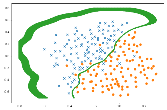
3.2 using the selected parameters and Gaussian kernel SVM applied to the data set 3

In [136]:

svc = svm.SVC(C=best_C, gamma=best_gamma)
svc.fit(X, y)

x1, x2 = find_decision_boundary(svc, -0.8, 0.3, -0.7, 0.8, 0.005)
fig, ax = plt.subplots(figsize=(9,6))
plot_init_data(data, fig, ax)
ax.scatter(x1, x2, s=5)
plt.show()

4 apply SVM to handwritten numeral recognition

In this part of the experiment, linear SVM and Gaussian kernel SVM are applied to handwritten dataset: UCI ml hand written digits datasets, and the recognition results are compared.

In [137]:

# Import the required library files
from sklearn import datasets, svm, metrics
from sklearn.model_selection import train_test_split

In [138]:

# Download the dataset from the sklearn library and show some samples
digits = datasets.load_digits()

_, axes = plt.subplots(1, 10) 
images_and_labels = list(zip(digits.images, digits.target))
for ax, (image, label) in zip(axes, images_and_labels[0:10]):
    ax.set_axis_off()
    ax.imshow(image, cmap=plt.cm.gray_r, interpolation='nearest')
    ax.set_title(' %i' % label)
plt.show()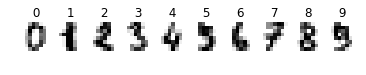

In [139]:

Turn each picture sample into a vector
n_samples = len(digits.images)
data = digits.images.reshape((n_samples, -1))

# Divide the original data set into training set and test set (half training and the other half testing)
X_train, X_test, y_train, y_test = train_test_split(
    data, digits.target, test_size=0.5, shuffle=False)#False

**Key point 5: * * the task of this part is * * to apply linear SVM (C=1) and Gaussian kernel SVM (C=1, gamma=0.001) to UCI handwritten dataset and output recognition accuracy**

In [140]:

#The linear SVM is applied to the data set and the recognition results are output
# ======================Fill in the code here======================= 
svc = svm.SVC(kernel="linear")
svc.fit(X_train, y_train)
score_Linear=svc.score(X_test, y_test) 
# ============================================================= 

print("Classification accuracy of Linear SVM:", score_Linear)

Classification accuracy of Linear SVM: 0.9443826473859844

In [141]:

#The linear SVM is applied to the data set and the recognition results are output
# ======================Fill in the code here======================= 
svc = svm.SVC(kernel="linear")
svc.fit(X_train, y_train)
score_Linear=svc.score(X_test, y_test) 
# ============================================================= 

print("Classification accuracy of Linear SVM:", score_Linear)

Classification accuracy of Gaussian SVM: 0.9688542825361512

Posted by egturnkey on Fri, 15 Oct 2021 11:55:14 -0700

Programmer Group