Come and explore happiness together (complete)

This learning note is the learning content of Alibaba cloud Tianchi Longzhu plan machine learning training camp. The learning links are: AI training camp machine learning - Alibaba cloud Tianchi

• Introduction to the game title (although there is already an introduction to the game title in the above link, I still excerpted it. It is definitely not water word count (manual dog head))
• Understand the data, and conduct preliminary exploration and visualization
• Characteristic Engineering
• Model building

Special note: as I am still shallow in knowledge, in order to improve the accuracy, I refer to the works of some forum friends in the model building part. I would like to thank them for their sharing.

When using the code, I also annotate my understanding when learning. If you are also the first time to contact these modules, you may be able to help.

1, Introduction to competition questions

Competition background
In the field of social science, the research of well-being occupies an important position. This topic involving philosophy, psychology, sociology, economics and other disciplines is complex and interesting; At the same time, it is closely related to everyone's life. Everyone has his own measure of happiness. If we can find the commonness that affects happiness, will life be more fun; If we can find the policy factors affecting happiness, we can optimize the allocation of resources to improve people's happiness. At present, social science research focuses on the interpretability of variables and the implementation of future policies, mainly using the methods of linear regression and logical regression, in terms of economic and demographic factors such as income, health, occupation, social relations and leisure style; And government public services, macroeconomic environment, tax burden and other macro factors.
I tried The classic topic of well-being prediction hopes to have algorithm attempts in other dimensions in addition to the existing social science research, combine the respective advantages of multiple disciplines, tap the potential influencing factors, and find more interpretable and understandable relationships.
Description of competition questions
The competition questions use the questionnaire survey results of public data, and select multiple groups of variables, including Individual variables (gender, age, region, occupation, health, marriage and political outlook, etc.) Family variables (parents, spouses, children, family capital, etc.) Social attitudes (fairness, credit, public service, etc.) to predict their impact on Evaluation of well-being.
The accuracy of well-being prediction is not the only purpose of the competition, but also hopes that players can explore and harvest the relationship between variables and the significance of variable groups.
Data description
Considering the large number of variables and the complex relationship between some variables, the data is divided into Full version and There are two types of compact version. You can start with the simplified version, get familiar with the competition questions, and use the full version to mine more information. The complete file is the variable full version data, and the abbr file is the variable reduced version data.
The index file contains the questionnaire title corresponding to each variable and the meaning of variable value.
The survey file is the original questionnaire of the data source as a supplement to facilitate the understanding of the problem background.
Data source: the data used in the competition comes from the China Comprehensive Social Survey (CGSS) project hosted by the China Survey and data center of Renmin University of China. The competition thanks this organization and its personnel for providing data assistance. China comprehensive social survey Multistage stratified sampling Cross sectional interview survey.
External data: the competition takes data mining and analysis as the starting point and does not restrict the use of external data, such as public data such as macroeconomic indicators and government redistribution policies. Players are welcome to exchange and share.
Evaluation index
The submission result is a csv file, which contains two columns: the predicted value of id and happiness.
Score calculation formula:
 
Where n represents the number of samples in the test set, yi represents the predicted value of the ith sample, and y * represents the real value.

Please go to Alibaba cloud Tianchi to obtain data related to the competition

Come and explore happiness together! Competition questions and data - Tianchi competition - Alibaba cloud Tianchi} tianchi.aliyun.com/competition/entry/231702/information uploading... Re uploading cancelled

2. Data processing

# Import the packages needed for the entire project
import os
import time 
import pandas as pd
import numpy as np
import lightgbm as lgb # A machine learning algorithm can improve the accuracy of prediction
import seaborn as sns
from sklearn.metrics import roc_auc_score, roc_curve # Calculate the value of the area under the roc curve
from sklearn.model_selection import KFold  # k-fold cross analysis
from sklearn.model_selection import train_test_split
from sklearn.linear_model import LogisticRegression
from sklearn.svm import SVC, LinearSVC 
from sklearn.ensemble import RandomForestClassifier
from sklearn.neighbors import KNeighborsClassifier
from sklearn.naive_bayes import GaussianNB
from sklearn.linear_model import Perceptron
from sklearn.linear_model import SGDClassifier
from sklearn.tree import DecisionTreeClassifier
from sklearn.model_selection import GridSearchCV
from sklearn import metrics
from sklearn.metrics import mean_squared_error # Mean square error

# 1. Load data

train = pd.read_csv("happiness_train_complete.csv", parse_dates=["survey_time"], encoding='latin-1') 
test = pd.read_csv("happiness_test_complete.csv", parse_dates=["survey_time"], encoding='latin-1')
train.head()

# 2. Understanding data sets

# View the data distribution of features
train.describe()

# Delete the data corresponding to invalid labels in the training set
train = train.loc[train['happiness'] != -8]

# Check the distribution of each category. It is obvious that the category is unbalanced
f,ax=plt.subplots(1,2,figsize=(18,8))
train['happiness'].value_counts().plot.pie(autopct='%1.1f%%',ax=ax[0],shadow=True)
ax[0].set_title('happiness')
ax[0].set_ylabel('')
train['happiness'].value_counts().plot.bar(ax=ax[1])
ax[1].set_title('happiness')
plt.show()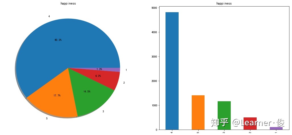

# Explore the distribution of gender and happiness
sns.countplot('gender',hue='happiness',data=train)
ax[1].set_title('Sex:happiness')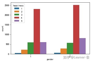

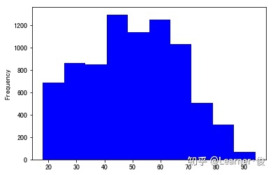
# Explore the relationship between age and happiness
train['survey_time'] = train['survey_time'].dt.year
test['survey_time'] = test['survey_time'].dt.year
train['Age'] = train['survey_time']-train['birth']
test['Age'] = test['survey_time']-test['birth']
del_list=['survey_time','birth']
figure,ax = plt.subplots(1,1)
train['Age'].plot.hist(ax=ax,color='blue')

# Generally, age is divided into boxes to avoid the influence of noise and outliers
combine=[train,test]

for dataset in combine:
    dataset.loc[dataset['Age']<=16,'Age']=0
    dataset.loc[(dataset['Age'] > 16) & (dataset['Age'] <= 32), 'Age'] = 1
    dataset.loc[(dataset['Age'] > 32) & (dataset['Age'] <= 48), 'Age'] = 2
    dataset.loc[(dataset['Age'] > 48) & (dataset['Age'] <= 64), 'Age'] = 3
    dataset.loc[(dataset['Age'] > 64) & (dataset['Age'] <= 80), 'Age'] = 4
    dataset.loc[ dataset['Age'] > 80, 'Age'] = 5
sns.countplot('Age', hue='happiness', data=train)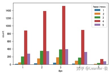

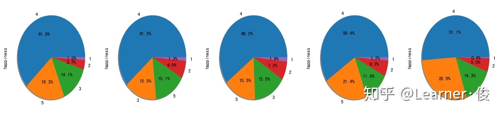
figure1,ax1 = plt.subplots(1,5,figsize=(18,4))
train['happiness'][train['Age']==1].value_counts().plot.pie(autopct='%1.1f%%',ax=ax1[0],shadow=True)
train['happiness'][train['Age']==2].value_counts().plot.pie(autopct='%1.1f%%',ax=ax1[1],shadow=True)
train['happiness'][train['Age']==3].value_counts().plot.pie(autopct='%1.1f%%',ax=ax1[2],shadow=True)
train['happiness'][train['Age']==4].value_counts().plot.pie(autopct='%1.1f%%',ax=ax1[3],shadow=True)
train['happiness'][train['Age']==5].value_counts().plot.pie(autopct='%1.1f%%',ax=ax1[4],shadow=True)

# feature selection 
# At present, only feature selection through correlation is considered
train.corr()['happiness'][abs(train.corr()['happiness'])>0.05]

happiness 1.000000
edu 0.103048
edu_yr 0.055564
political 0.080986
join_party 0.069007
property_8 -0.051929
weight_jin 0.085841
health 0.250538
health_problem 0.186620
depression 0.304973
hukou 0.072936
media_1 0.095035
media_2 0.084872
media_3 0.091431
media_4 0.098809
media_5 0.065220
media_6 0.059273
leisure_1 -0.077097
leisure_3 -0.070262
leisure_4 -0.095676
leisure_6 -0.107672
leisure_7 -0.072011
leisure_8 -0.100313
leisure_9 -0.148888
leisure_12 -0.068778
socialize 0.082206
relax 0.113233
learn 0.108294
social_friend -0.091079
socia_outing 0.059567
...
family_income 0.051506
family_m 0.061062
family_status 0.204702
house 0.089261
car -0.085387
invest_1 -0.055013
invest_2 0.054019
s_edu 0.125679
s_political 0.068802
s_hukou 0.071953
status_peer -0.150246
status_3_before -0.076808
view 0.078986
trust_1 0.069830
trust_2 0.054909
trust_5 0.102110
trust_7 0.060102
trust_8 0.065644
trust_10 0.069740
trust_12 0.057885
neighbor_familiarity 0.054074
public_service_1 0.112537
public_service_2 0.126029
public_service_3 0.134028
public_service_4 0.129880
public_service_5 0.136347
public_service_6 0.162514
public_service_7 0.154029
public_service_8 0.128678
public_service_9 0.129723
Name: happiness, Length: 65, dtype: float64

# Select the features with correlation greater than 0.05 as candidate features to participate in the training, and add the features we think are more important. A total of 66 features participate in the training
features = (train.corr()['happiness'][abs(train.corr()['happiness'])>0.05]).index
features = features.values.tolist()
features.extend(['Age', 'work_exper'])
features.remove('happiness')
len(features)

3. Model building

# Generate data and labels
target = train['happiness']
train_selected = train[features]
test = test[features]
feature_importance_df = pd.DataFrame()
oof = np.zeros(len(train))
predictions = np.zeros(len(test))

# The following params are mainly parameter adjustment
params = {'num_leaves': 9,
         'min_data_in_leaf': 40,
         'objective': 'regression',
         'max_depth': 16,
         'learning_rate': 0.01,
         'boosting': 'gbdt',
         'bagging_freq': 5,
         'bagging_fraction': 0.8,   # Data scale used for each iteration
         'feature_fraction': 0.8201,# In each iteration, 80% of the parameters are randomly selected to build the tree
         'bagging_seed': 11,
         'reg_alpha': 1.728910519108444,
         'reg_lambda': 4.9847051755586085,
         'random_state': 42,
         'metric': 'rmse',
         'verbosity': -1,
         'subsample': 0.81,
         'min_gain_to_split': 0.01077313523861969,
         'min_child_weight': 19.428902804238373,
         'num_threads': 4}


kfolds = KFold(n_splits=5,shuffle=True,random_state=15)
predictions = np.zeros(len(test))

for fold_n,(trn_index,val_index) in enumerate(kfolds.split(train_selected,target)):
    print("fold_n {}".format(fold_n))
    trn_data = lgb.Dataset(train_selected.iloc[trn_index],label=target.iloc[trn_index])
    val_data = lgb.Dataset(train_selected.iloc[val_index],label=target.iloc[val_index])
    num_round=10000
    clf = lgb.train(params, trn_data, num_round, valid_sets = [trn_data, val_data], verbose_eval=1000, early_stopping_rounds = 100)
    oof[val_index] = clf.predict(train_selected.iloc[val_index], num_iteration=clf.best_iteration)
    predictions += clf.predict(test,num_iteration=clf.best_iteration)/5
    fold_importance_df = pd.DataFrame()
    fold_importance_df["feature"] = features
    fold_importance_df["importance"] = clf.feature_importance()
    fold_importance_df["fold"] = fold_n + 1
    feature_importance_df = pd.concat([feature_importance_df, fold_importance_df], axis=0)
    print("CV score: {:<8.5f}".format(mean_squared_error(target, oof)**0.5))

fold_n 0
Training until validation scores don't improve for 100 rounds.
Early stopping, best iteration is:
[835] training's rmse: 0.631985 valid_1's rmse: 0.681313
CV score: 3.54967
fold_n 1
Training until validation scores don't improve for 100 rounds.
[1000] training's rmse: 0.618499 valid_1's rmse: 0.691913
Early stopping, best iteration is:
[1035] training's rmse: 0.616785 valid_1's rmse: 0.691461
CV score: 3.10335
fold_n 2
Training until validation scores don't improve for 100 rounds.
[1000] training's rmse: 0.629692 valid_1's rmse: 0.649479
Early stopping, best iteration is:
[1545] training's rmse: 0.605341 valid_1's rmse: 0.64739
CV score: 2.55891
fold_n 3
Training until validation scores don't improve for 100 rounds.
Early stopping, best iteration is:
[865] training's rmse: 0.62686 valid_1's rmse: 0.699352
CV score: 1.87169
fold_n 4
Training until validation scores don't improve for 100 rounds.
[1000] training's rmse: 0.62042 valid_1's rmse: 0.685821
Early stopping, best iteration is:
[1460] training's rmse: 0.600172 valid_1's rmse: 0.684194
CV score: 0.68097

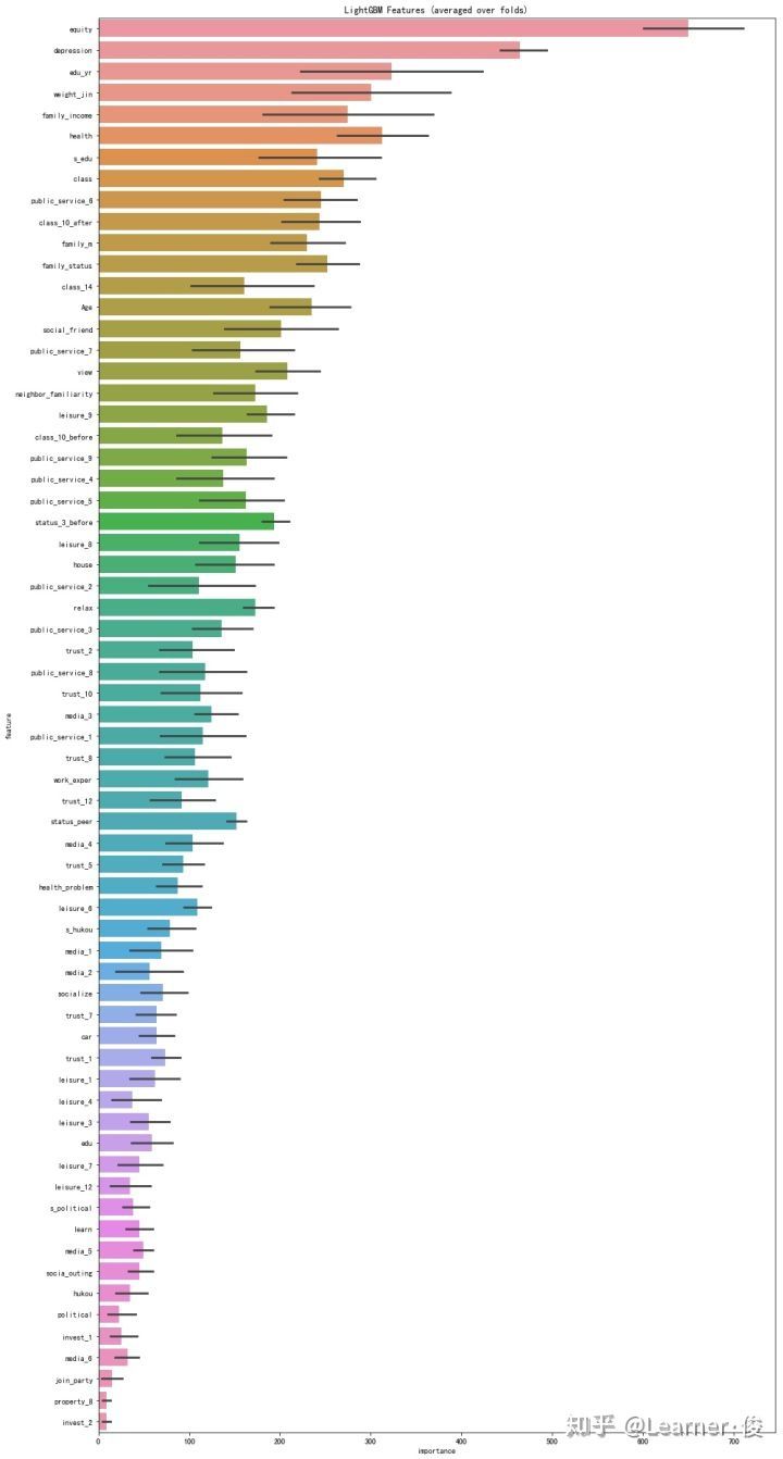
cols = (feature_importance_df[["feature", "importance"]]
        .groupby("feature")
        .mean()
        .sort_values(by="importance", ascending=False)[:1000].index)
best_features = feature_importance_df.loc[feature_importance_df.feature.isin(cols)]

plt.figure(figsize=(14,26))
sns.barplot(x="importance", y="feature", data=best_features.sort_values(by="importance",ascending=False))
plt.title('LightGBM Features (averaged over folds)')
plt.tight_layout()