preface
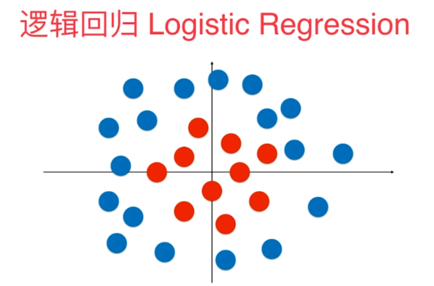
The essence of logistic regression mentioned in the previous blog is to find a straight line on the plane and use this straight line to segment the classification corresponding to all samples. Therefore, in most cases, logistic regression can only solve the dichotomous problem, because this straight line can only divide our plane into two parts. However, even so, we will find that the classification method of straight line is too simple. There are many other situations that cannot be classified simply by straight line. For example, in the figure below, some sample points are distributed in our feature plane. Red belongs to one category and blue belongs to another category. For these sample points, we can't divide them into two parts by straight line, Because the distribution of these sample points is nonlinear.
1, Basic idea of using polynomial features in logistic regression
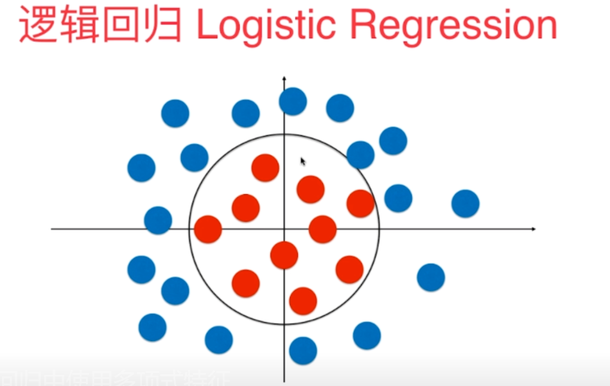
In fact, through observation, we can see that these sample points can be divided into two parts through a circular decision boundary. But the method we implemented before is that there is no way to get such a circular decision boundary.
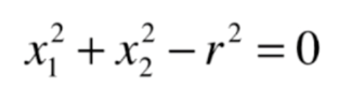
The equation of a general circle is shown in the figure below
Next, our idea is whether we can let our logistic regression learn such a boundary. In fact, we only introduce polynomial terms here.
The general meaning is that we regard the whole of x12 and x22 here as features, so the coefficient in front of x12 here is 1, and the coefficient in front of x22 is also 1, corresponding to our intercept θ 0 is - r2. The decision boundary obtained here is still a linear decision boundary for x12 and x22, but it becomes a nonlinear circular boundary for x1 and x2. In other words, we can transform the idea from linear regression to polynomial regression. Similarly, we can add polynomial terms to our logistic regression algorithm. Based on this way, we can get a good classification of nonlinear data and the decision boundary of the curve (a special circle is given here, and the coefficients of x12 and x22 can also be changed. By introducing different x1 and X2, we can get the circle or ellipse with the center of the circle at different positions).
2, Implementation process
1. Draw sample points
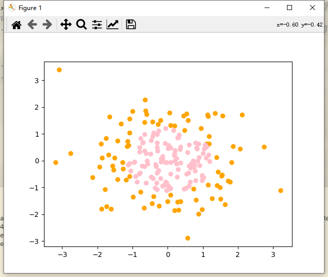
import numpy as np
import matplotlib.pyplot as plt

np.random.seed(666) # Add random seed
X = np.random.normal(0, 1, size=(200, 2)) # Random sequence with mean value of 0 and standard deviation of 1. 200 samples, 2 features per sample
# Boolean type is converted to int type. true corresponds to 1 and false corresponds to 0
y = np.array(X[:, 0]**2 + X[:, 1]**2 < 1.5, dtype='int') # Square of the first feature (first column) of X + square of the second feature (second column) of X, radius value 1.5

# Draw sample
plt.scatter(X[y == 0, 0], X[y == 0, 1], color = "orange")
plt.scatter(X[y == 1, 0], X[y == 1, 1], color = "pink")
plt.show()
Set 200 samples with 2 features for each sample, and classify x2 + Y2 < 1.5, that is, the points inside the circle (pink points) are classified as 1, and the points outside the circle (orange points) are classified as 0
2. Instantiate object
Before instantiation, let's use the class of logical regression mentioned in the blog again. Let's put it out here
# Logistic regression class
class logisticsRegression:
  def __init__(self):
      # Initialize the logistics Regression model
      self.coef_ = None # The coefficient corresponds to theta1-n, the corresponding vector
      self.interception_ = None # Intercept, corresponding to theta0
      self._theta = None # Define private variables and calculate theta as a whole

  # sigmoid function data overflow: https://blog.csdn.net/wofanzheng/article/details/103976889
  # Define private sigmoid function
  # def _sigmoid(self, t):
  #   return 1. / 1. + np.exp(-t)

  def _sigmoid(self, x):
    l=len(x)
    y=[]
    for i in range(l):
      if x[i]>=0:
        y.append(1.0/(1+np.exp(-x[i])))
      else:
        y.append(np.exp(x[i])/(np.exp(x[i])+1))
    return y

  '''
    gradient descent
  '''
  def fit(self, X_train, y_train, eta = 5.0, n_iters = 1e4):
    # According to training data set X_train, y_ .train training logistics Regression model
    # X_ Sample number and y of train_ The number of tags in the train should be consistent
    # Use shape[0] to read the length of the first dimension of the matrix, here is the number of columns
    assert X_train.shape[0] == y_train.shape[0], \
    "the size of x_ .train must be equal to the size of y_ train"
    # loss function
    def J(theta, X_b, y):
      y_hat = self._sigmoid(X_b.dot(theta))
      try:
        return -np.sum(y * np.log(y_hat) + (1 - y) * np.log(1 - y_hat)) / len(y)
      except:
        return float('inf') # Returns the maximum float value

    # Gradient (more stupid method)
    def dJ(theta, X_b, y):
      return X_b.T.dot(self._sigmoid(X_b.dot(theta)) - y) / len(X_b)


    # Solving theta matrix by gradient descent
    def gradient_descent(X_b, y, initial_theta, eta, n_iters = 1e4, epsilon = 1e-8):
      theta = initial_theta
      cur_iters = 0

      while cur_iters < n_iters:
          gradient = dJ(theta, X_b, y) # Find gradient
          last_theta = theta # Before theta is reassigned, record the value of the previous field
          theta = theta - eta * gradient # Obtain theta of the next point through a certain eta learning rate
          # If the difference of the loss function between the nearest two points is less than a certain accuracy, exit the cycle
          if(abs(J(theta, X_b, y) - J(last_theta, X_b, y)) < epsilon):
              break
          cur_iters += 1
      return theta

    # Get X_b
    X_b = np.hstack([np.ones((len(X_train), 1)), X_train])
    initial_theta = np.zeros(X_b.shape[1]) # Set the vector of n+1 dimension, X_b.shape[1]: Dimension of the first row
    # X_b.T is X_ Transpose of B,. Dot is dot multiplication and np.linalg.inv is inverse
    # Get theta
    self._theta = gradient_descent(X_b, y_train, initial_theta, eta, n_iters)

    self.interception_ = self._theta[0] # intercept
    self.coef_ = self._theta[1:] # coefficient
    return self

  '''
    Process of predicting possibility
  '''
  def predict_prob(self, X_predict):
    # Given data set to be predicted X_predict, return x_ Result probability vector of predict
    X_b = np.hstack([np.ones((len(X_predict), 1)), X_predict])
    return self._sigmoid(X_b.dot(self._theta))


  '''
    Prediction process
  '''
  def predict(self, X_predict):
    # Given data set to be predicted X_predict, return x_ Result vector of predict
    prob = self.predict_prob(X_predict) # The prob vector stores floating-point numbers of 0-1
    # Classify (boolean type cast to integer)
    # return np.array(prob >= 0.5, dtype='int')
    l = len(prob)
    temp_prob=[]
    for i in range(l):
      if prob[i] >= 0.5:
        temp_prob.append(1)
      else:
        temp_prob.append(0)
    return temp_prob

  '''
    Display properties
  '''
  def __repr__(self):
      return "logisticsRegression()"
Here, the whole part of the content can be encapsulated into a single file, which can be directly imported every time it needs to be instantiated
from classLogisticsRegression import logisticsRegression # Introduce logistic regression objects
Then instantiate
log_reg = logisticsRegression()
3. Add method for drawing decision boundary
'''
  Draw decision boundaries
  params-model:Trained model
  params-axis:Drawing area axis range (0),1,2,3 corresponding x Shaft and y Range of axes)
'''
def plot_decision_boundary(model, axis):
  # meshgrid: generate grid point coordinate matrix
  x0, x1 = np.meshgrid(
    # Divide the x-axis into countless points through linspace
    # axis[1] - axis[0] is the left boundary of x minus the right boundary of X
    # axis[3] - axis[2]: the maximum value of y minus the minimum value of y

    # arr.shape    # (a,b)
    # arr.reshape(m,-1) #Change the dimension to m rows and D columns (- 1 means the number of columns is calculated automatically, d= a*b /m)
    # arr.reshape(-1,m) #Change the dimension to row D and column m (- 1 means the number of rows is calculated automatically, d= a*b /m)
    np.linspace(axis[0], axis[1], int((axis[1] - axis[0]) * 100)).reshape(-1, 1),
    np.linspace(axis[2], axis[3], int((axis[3] - axis[2]) * 100)).reshape(-1, 1),
  )
  print('x0', x0)
  # print('x1', x1)
  # np.r_ It is to connect two matrices by column, that is, add the two matrices up and down. The number of columns is required to be equal, and the number of columns remains unchanged after adding.
  # np.c_ It is to connect two matrices by row, that is, add the left and right of the two matrices. The number of rows is required to be equal, and the number of rows remains unchanged after adding.
  # . t ravel(): convert multidimensional array to one-dimensional array
  X_new = np.c_[x0.ravel(), x1.ravel()]
  y_predict = model.predict(X_new)

  # ZZ = y is not allowed here_ Predict.reshape (x0. Shape), the error 'list' object has no attribute 'reshape' will be reported
  # To convert through np.array
  zz = np.array(y_predict).reshape(x0.shape)

  from matplotlib.colors import ListedColormap
  # ListedColormap allows users to define their desired color library using hexadecimal color codes and appears as the cmap parameter in plt.scatter():
  custom_cmap = ListedColormap(['#F5FFFA', '#FFF59D', '#90CAF9'])
  # coutourf([X, Y,] Z,[levels], **kwargs),contourf draws the area between the climbing lines
  # Z is an array with the same dimension as X and y.
  plt.contourf(x0, x1, zz, linewidth=5, cmap=custom_cmap)
4. Draw decision boundary and sample points
# Training samples and test samples are not divided here. All samples are directly used for training
log_reg.fit(X, y)
# Draw decision boundaries
plot_decision_boundary(log_reg, axis=[-4, 4, -4, 4]) # x. The range of the y-axis is roughly (- 4,4)
# Draw sample
plt.scatter(X[y == 0, 0], X[y == 0, 1], color = "orange")
plt.scatter(X[y == 1, 0], X[y == 1, 1], color = "pink")
plt.show()
Decision boundary and sample points
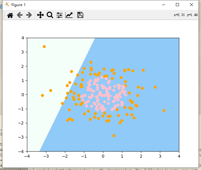
The previous logistic regression algorithm itself uses a straight line to divide our feature plane. Obviously, there are many errors in dividing our sample points in our plane. Next, we implement it with the help of pipeline pipeline.
5. Implementation of polynomial regression with pipeline
Before that, the class of previous logistic regression is encapsulated separately and then introduced for use
Logistic regression class
# Logistic regression class

import numpy as np
from sklearn.metrics import accuracy_score


class logisticsRegression:
  def __init__(self):
      # Initialize the logistics Regression model
      self.coef_ = None # The coefficient corresponds to theta1-n, the corresponding vector
      self.interception_ = None # Intercept, corresponding to theta0
      self._theta = None # Define private variables and calculate theta as a whole

  # sigmoid function data overflow: https://blog.csdn.net/wofanzheng/article/details/103976889
  # Define private sigmoid function
  # def _sigmoid(self, t):
  #   return 1. / 1. + np.exp(-t)

  def _sigmoid(self, x):
    l=len(x)
    y=[]
    for i in range(l):
      if x[i]>=0:
        y.append(1.0/(1+np.exp(-x[i])))
      else:
        y.append(np.exp(x[i])/(np.exp(x[i])+1))
    return y

  '''
    gradient descent
  '''
  def fit(self, X_train, y_train, eta = 5.0, n_iters = 1e4):
    # According to training data set X_train, y_ .train training logistics Regression model
    # X_ Sample number and y of train_ The number of tags in the train should be consistent
    # Use shape[0] to read the length of the first dimension of the matrix, here is the number of columns
    assert X_train.shape[0] == y_train.shape[0], \
    "the size of x_ .train must be equal to the size of y_ train"
    # loss function
    def J(theta, X_b, y):
      y_hat = self._sigmoid(X_b.dot(theta))
      try:
        return -np.sum(y * np.log(y_hat) + (1 - y) * np.log(1 - y_hat)) / len(y)
      except:
        return float('inf') # Returns the maximum float value

    # Gradient (more stupid method)
    def dJ(theta, X_b, y):
      return X_b.T.dot(self._sigmoid(X_b.dot(theta)) - y) / len(X_b)


    # Solving theta matrix by gradient descent
    def gradient_descent(X_b, y, initial_theta, eta, n_iters = 1e4, epsilon = 1e-8):
      theta = initial_theta
      cur_iters = 0

      while cur_iters < n_iters:
          gradient = dJ(theta, X_b, y) # Find gradient
          last_theta = theta # Before theta is reassigned, record the value of the previous field
          theta = theta - eta * gradient # Obtain theta of the next point through a certain eta learning rate
          # If the difference of the loss function between the nearest two points is less than a certain accuracy, exit the cycle
          if(abs(J(theta, X_b, y) - J(last_theta, X_b, y)) < epsilon):
              break
          cur_iters += 1
      return theta

    # Get X_b
    X_b = np.hstack([np.ones((len(X_train), 1)), X_train])
    initial_theta = np.zeros(X_b.shape[1]) # Set the vector of n+1 dimension, X_b.shape[1]: Dimension of the first row
    # X_b.T is X_ Transpose of B,. Dot is dot multiplication and np.linalg.inv is inverse
    # Get theta
    self._theta = gradient_descent(X_b, y_train, initial_theta, eta, n_iters)

    self.interception_ = self._theta[0] # intercept
    self.coef_ = self._theta[1:] # coefficient
    return self

  '''
    Process of predicting possibility
  '''
  def predict_prob(self, X_predict):
    # Given data set to be predicted X_predict, return x_ Result probability vector of predict
    X_b = np.hstack([np.ones((len(X_predict), 1)), X_predict])
    return self._sigmoid(X_b.dot(self._theta))


  '''
    Prediction process
  '''
  def predict(self, X_predict):
    # Given data set to be predicted X_predict, return x_ Result vector of predict
    prob = self.predict_prob(X_predict) # The prob vector stores floating-point numbers of 0-1
    # Classify (boolean type cast to integer)
    # return np.array(prob >= 0.5, dtype='int')
    l = len(prob)
    temp_prob=[]
    for i in range(l):
      if prob[i] >= 0.5:
        temp_prob.append(1)
      else:
        temp_prob.append(0)
    return temp_prob
  '''
    Prediction accuracy
  '''
  def score(self, X_test, y_test):
    # According to test data set X_test and y_test determines the accuracy of the current model
    y_predict = self.predict(X_test)
    return accuracy_score(y_test, y_predict)

  '''
    Display properties
  '''
  def __repr__(self):
      return "logisticsRegression()"
Polynomial regression of pipeline packaging
from classLogisticsRegression import logisticsRegression # Introduce logistic regression objects
from sklearn.pipeline import Pipeline
from sklearn.preprocessing import PolynomialFeatures, StandardScaler

# Package pipeline for polynomial regression (pass in degree and return the class of polynomial regression)
def PolynomialLogisticsRegression(degree):
  # Use pipeline to create a pipeline and send it to poly_ The data of the reg object will be processed in sequence along the three steps of the pipeline
  return Pipeline([ # Pipeline passes in a list, in which the class corresponding to each step in the pipeline is passed in (this class is transmitted in the form of tuples)
    ("poly", PolynomialFeatures(degree=degree)), # Step 1: find polynomial features, which is equivalent to poly = PolynomialFeatures(degree=2)
    ("std_scaler", StandardScaler()), # Step 2: numerical homogenization
    ("log_reg", logisticsRegression()) # Step 3: perform logistic regression
  ])

poly_log_reg = PolynomialLogisticsRegression(2)
poly_log_reg.fit(X, y)
# Query classification accuracy
print('Classification accuracy', poly_log_reg.score(X, y))
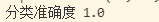
You can see that the classification accuracy is very high.
Next, draw the decision boundary
# Draw decision boundaries
plot_decision_boundary(log_reg, axis=[-4, 4, -4, 4]) # x. The range of the y-axis is roughly (- 4,4)
# Draw sample
plt.scatter(X[y == 0, 0], X[y == 0, 1], color = "orange")
plt.scatter(X[y == 1, 0], X[y == 1, 1], color = "pink")
plt.show()
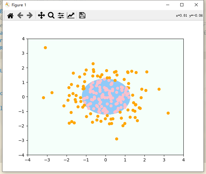
After drawing the decision boundary, we can see that the decision boundary is equivalent to a circle, which can well divide the nonlinear data. However, in fact, the data encountered cannot be so round. If it is a very strange parameter, our degree must select other values accordingly. Next, try degree to select other values.
degree=20
''' degree=20 '''
poly_log_reg2 = PolynomialLogisticsRegression(20)
poly_log_reg2.fit(X, y)
# Query classification accuracy
print('degree=20 Classification accuracy', poly_log_reg2.score(X, y))
# Draw decision boundaries
plot_decision_boundary(poly_log_reg2, axis=[-4, 4, -4, 4]) # x. The range of the y-axis is roughly (- 4,4)
# Draw sample
plt.scatter(X[y == 0, 0], X[y == 0, 1], color = "orange")
plt.scatter(X[y == 1, 0], X[y == 1, 1], color = "pink")
plt.show()
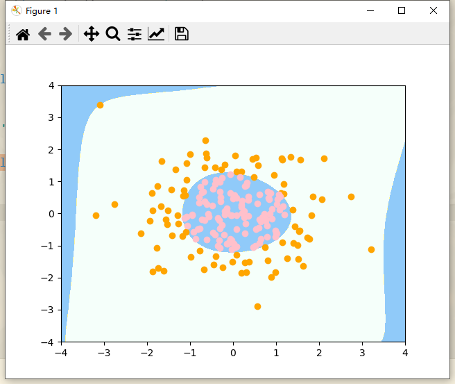
Outside the image, the decision boundary is very strange. In fact, the peripheral boundary is not what we want. This occurs because our degree=20 is too large, resulting in irregular shape. In this case, it belongs to over fitting.
The idea of solving over fitting: the simplest is to reduce the value of degree, and the other is to regularize the model.