5.1 Basic operations
5.2 Moving data around
5.3 Computing on data
5.4 Plotting data
5.5 For while if statement and functions
5.6 Vectorization
After reading the first two lessons, I think matlab seems to be the same as octave, so I plan to use matlab to learn the fifth lesson
basic operation
?? Ugly...
>> 5 + 6

ans =        % matlab Command line ans That's what it looks like. Take up the space. I'm not willing to change the format qaq

    11

>> 3 - 2

ans =

     1

>> 5 * 8

ans =

    40

>> 2^6

ans =

    64

>> 1 == 2    %false

ans =

     0

>> 1 ~= 2     %true  [notes] This is not writing ~= Instead of !=  (Different from other programming languages)

ans =

     1

>> 1 && 0    %AND

ans =

     0

>> 1 || 0   %OR

ans =

     1

>> xor(1,0)

ans =

     1
variable
>> a = 3

a =

     3

>> a = 3;           %  semicolon ";" supressing output  No output a
>> b = 'hi';
>> c = (3 >= 1);
>> c

c =

     1

>> b

b =

hi

>> a = pi;
>> a

a =

    3.1416

>> disp(a)                %disp
    3.1416

>> disp(sprintf('2 decimals: %0.2f', a))
2 decimals: 3.14

>> disp(sprintf('6 decimals: %0.6f', a))
6 decimals: 3.141593

>> format long            %format
>> a

a =

   3.141592653589793

>> format short
>> a

a =

    3.1416
Vector sum matrix
>> A = [1 2; 3 4; 5 6]
A =
1 2
3 4
5 6
>> A = [1 2; %Another input matrix A Way
3 4;
5 6]
A =
1 2
3 4
5 6
>> v = [ 1 2 3] %Row vector
v =
1 2 3
>> v = [1; 2; 3] %Column vector
v =
1
2
3
>> v = 1: 0.1: 2 %0 steps from 1 to 2.1
v =
1.0000 1.1000 1.2000 1.3000 1.4000 1.5000 1.6000 1.7000 1.8000 1.9000 2.0000
>> v = 1 : 6
v =
1 2 3 4 5 6
>> ones (2, 3) %ones All 1 matrices
ans =
1 1 1
1 1 1
>> C = 2*ones(2, 3)
C =
2 2 2
2 2 2
>> w = zeros(1, 3) %zeros All 0 matrices
w =
0 0 0
>> w = rand(1, 3) %rand 0~1 random number
w =
0.8147 0.9058 0.1270
>> w = rand(3, 3)
w =
0.9134 0.2785 0.9649
0.6324 0.5469 0.1576
0.0975 0.9575 0.9706
>> w = randn(1, 3) %randn Gauss random number
w =
0.7254 -0.0631 0.7147
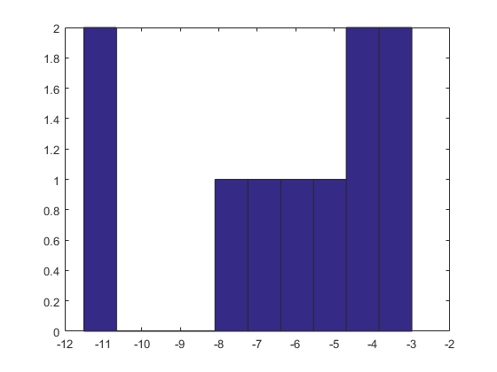
>> w = -6 + sqrt(10)*(randn(1, 10));
>> w
w =
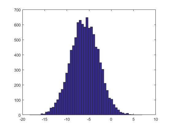
-5.6077 -1.4568 -12.2009 -6.6252 -9.8195 3.1959 -3.3904 -1.6393 -9.3463 -7.4819
>> hist(w) %hist Draw w Histogram of (figure given after code)
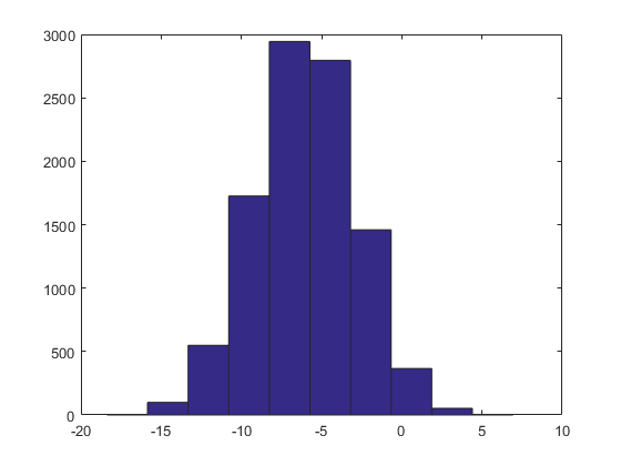
>> w = -6 + sqrt(10)*(randn(1, 100));
>> hist(w)
>> w = -6 + sqrt(10)*(randn(1, 10000));
>> hist(w)
>> hist(w,50) %Prescribed column number
>> eye(4) %eye Unit matrix
ans =
1 0 0 0
0 1 0 0
0 0 1 0
0 0 0 1
>> help eye %help File
eye Identity matrix.
eye(N) is the N-by-N identity matrix.
eye(M,N) or eye([M,N]) is an M-by-N matrix with 1's on
the diagonal and zeros elsewhere.
eye(SIZE(A)) is the same size as A.
eye with no arguments is the scalar 1.
eye(..., CLASSNAME) is a matrix with ones of class specified by
CLASSNAME on the diagonal and zeros elsewhere.
eye(..., 'like', Y) is an identity matrix with the same data type, sparsity,
and complexity (real or complex) as the numeric variable Y.
Note: The size inputs M and N should be nonnegative integers.
Negative integers are treated as 0.
Example:
x = eye(2,3,'int8');
See also speye, ones, zeros, rand, randn.
eye Reference page
//Other functions named eye
>>
w = -6 + sqrt(10)*(randn(1, 10));
w = -6 + sqrt(10)*(randn(1, 100));

w = -6 + sqrt(10)*(randn(1, 10000));
>> clear %Clear all variables in the workspace
>> A = [1 2;3 4; 5 6]
A =
1 2
3 4
5 6
>> size(A) %size matrix A Size
ans =
3 2
>> sz = size(A)
sz =
3 2
>> size(sz)
ans =
1 2
>> size(A, 1) %A The size of the first dimension of a matrix is the number of matrix rows
ans =
3
>> size(A, 2) %A The size of the second dimension of a matrix is the number of columns
ans =
2
>> v = [1 2 3 4]
v =
1 2 3 4
>> length(v) %Size of the largest dimension
ans =
4
>> length(A) %But in general length Mostly used to find vector length
ans =
3
>> length([1; 2; 3; 4; 5])
ans =
5
>> pwd %pwd current path
ans =
C:\Users\asus\Documents\MATLAB
>> cd 'C:\Users\asus\Desktop' %cd Modify path(To the desktop Desktop)
>> ls %ls Document under current path
2020winter Sublime Text 3.lnk lab01.zip
Adobe Dreamweaver CC 2018.lnk Typora.lnk
>> load featureX.dat
>> load priceY.dat
>> load('featureX.dat')
>> who %List all variables
//Your variable is% Chinese matlab
A ans featureX priceY sz v
>> whos %List all variable details
Name Size Bytes Class Attributes
A 3x2 48 double
ans 1x30 60 char
featureX 19x2 304 double
priceY 19x1 152 double
sz 1x2 16 double
v 1x4 32 double
>> featureX
featureX =
2104 3
1400 3
2400 3
1416 2
3000 4
1985 4
1534 3
1427 3
1330 3
1494 3
1940 4
2000 3
1890 3
4478 5
1238 3
2300 4
1320 2
1236 3
2609 4
>> size(featureX)
ans =
19 2
>> size(priceY)
ans =
19 1
>> clear featureX %Clear a variable
>> whos
Name Size Bytes Class Attributes
A 3x2 48 double
ans 1x2 16 double
priceY 19x1 152 double
sz 1x2 16 double
v 1x4 32 double
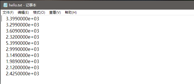
>> v = priceY(1:10) %take priceY First ten columns
v =
3399
3299
3609
2320
5399
2999
3149
1989
2120
2425
>> who
//Your variables are:
A ans priceY sz v
>> whos
Name Size Bytes Class Attributes
A 3x2 48 double
ans 1x2 16 double
priceY 19x1 152 double
sz 1x2 16 double
v 10x1 80 double
>> save hello.mat v; %save Storage file
>> clear
>> load hello.mat
>> whos
Name Size Bytes Class Attributes
v 10x1 80 double
>> v
v =
3399
3299
3609
2320
5399
2999
3149
1989
2120
2425
>> save hello.txt v -ascii %save as text(ASCII)
hello.txt
Indexes
>> A = [1 2; 3 4; 5 6]

A =

     1     2
     3     4
     5     6

>> A(3, 2)          %index

ans =

     6

>> A(2,:)          % ":" means every element along that row/column

ans =

     3     4

>> A(:,2)

ans =

     2
     4
     6

>> A([1 3], :)      %First and third lines

ans =

     1     2
     5     6

>> A(:,2) = [10; 11; 12]     %Replacement column

A =

     1    10
     3    11
     5    12

>> A = [A, [100; 101; 102]]    %append another column vector to the right

A =

     1    10   100
     3    11   101
     5    12   102

>> A(:)    %hold A Put all elements of into a column vector

ans =

     1
     3
     5
    10
    11
    12
   100
   101
   102

>> A = [1 2; 3 4; 5 6]

A =

     1     2
     3     4
     5     6

>> B = [11 12; 13 14; 15 16]

B =

    11    12
    13    14
    15    16

>> C = [A B]          %Left and right recombination

C =

     1     2    11    12
     3     4    13    14
     5     6    15    16

>> C = [A; B]         %Up and down reorganization

C =

     1     2
     3     4
     5     6
    11    12
    13    14
    15    16

>> size(C)

ans =

     6     2
>> A = [1 2; 3 4; 5 6]

A =

     1     2
     3     4
     5     6

>> B = [11 12; 13 14; 15 16]

B =

    11    12
    13    14
    15    16

>> C = [1 1; 2 2]

C =

     1     1
     2     2

>> A*C

ans =

     5     5
    11    11
    17    17

>> A .* B           %A,B Multiplication of corresponding elements   .General representation of operations between elements

ans =

    11    24
    39    56
    75    96

>> A

A =

     1     2
     3     4
     5     6

>> A .^ 2        %Here^ Space between and 2!

ans =

     1     4
     9    16
    25    36

>> v = [1; 2; 3]

v =

     1
     2
     3

>> 1 ./ v

ans =

    1.0000
    0.5000
    0.3333

>> 1 ./ A

ans =

    1.0000    0.5000
    0.3333    0.2500
    0.2000    0.1667

>> log(v)

ans =

         0
    0.6931
    1.0986

>> exp(v)

ans =

    2.7183
    7.3891
   20.0855

>> abs(v)

ans =

     1
     2
     3

>> abs([-1; -1; -3])

ans =

     1
     1
     3

>> -v

ans =

    -1
    -2
    -3

>> v + ones(length(v),1)           %Yes v Add one for each element in

ans =

     2
     3
     4

>> v + 1                  %Yes v Another way to add one to each element in

ans =

     2
     3
     4

>> A'              %Transposition

ans =

     1     3     5
     2     4     6

>> (A')'

ans =

     1     2
     3     4
     5     6

>> a = [1 15 2 0.5]

a =

    1.0000   15.0000    2.0000    0.5000

>> val = max(a)          %A Medium element maximum

val =

    15

>> [val, ind] = max(a)     %ind=index Location of index maximum element

val =

    15


ind =

     2

>> max(A)        %A Maximum for each column of

ans =

     5     6

>> a < 3         %a Each element of is compared with 3

ans =

     1     0     1     1

>> a

a =

    1.0000   15.0000    2.0000    0.5000

>> find(a < 3)      %Return value is its index value

ans =

     1     3     4

>> A = magic(3)        % magic The sum of elements in each row and column of a matrix is the same number

A =

     8     1     6
     3     5     7
     4     9     2

>> [r, c] = find( A >= 7)    %r=row  c=column

r =

     1
     3
     2


c =

     1
     2
     3

>> a

a =

    1.0000   15.0000    2.0000    0.5000

>> sum(a)

ans =

   18.5000

>> prod(a)      %Product of four elements

ans =

    15

>> floor(a)

ans =

     1    15     2     0

>> ceil(a)

ans =

     1    15     2     1

>> ceiling(a)
//Function or variable 'ceiling' is not defined.

%Andrew Ng The teacher said ceiling=ceil But in matlab No such command in may only apply to octave

>> rand(3)    %3*3 Random matrix

ans =

    0.0581    0.1216    0.3025
    0.3230    0.7500    0.6023
    0.8535    0.4727    0.2124

>> max(rand(3),rand(3))     %From two to 3*3 In the matrix, the

ans =

    0.6958    0.7344    0.7514
    0.8546    0.9334    0.9937
    0.3971    0.8652    0.4279

>> A

A =

     8     1     6
     3     5     7
     4     9     2

>> max(A,[],1)       %A Maximum value of each column of matrix

ans =

     8     9     7

>> max(A,[],2)      %A Maximum value of each row of matrix  max Calculate the maximum value of each column by default

ans =

     8
     7
     9

>> max(max(A))    %seek A Medium maximum element

ans =

     9

>> A(:)

ans =

     8
     3
     4
     1
     5
     9
     6
     7
     2

>> max(A(:))     %seek A Another method of maximum element in

ans =

     9

>> A = magic(9)

A =

    47    58    69    80     1    12    23    34    45
    57    68    79     9    11    22    33    44    46
    67    78     8    10    21    32    43    54    56
    77     7    18    20    31    42    53    55    66
     6    17    19    30    41    52    63    65    76
    16    27    29    40    51    62    64    75     5
    26    28    39    50    61    72    74     4    15
    36    38    49    60    71    73     3    14    25
    37    48    59    70    81     2    13    24    35

>> sum(A,1)  %take A Add each column of

ans =

   369   369   369   369   369   369   369   369   369

>> sum(A,2)    %take A Add each line of

ans =

   369
   369
   369
   369
   369
   369
   369
   369
   369

>> eye(9)

ans =

     1     0     0     0     0     0     0     0     0
     0     1     0     0     0     0     0     0     0
     0     0     1     0     0     0     0     0     0
     0     0     0     1     0     0     0     0     0
     0     0     0     0     1     0     0     0     0
     0     0     0     0     0     1     0     0     0
     0     0     0     0     0     0     1     0     0
     0     0     0     0     0     0     0     1     0
     0     0     0     0     0     0     0     0     1

>> A .* eye(9)

ans =

    47     0     0     0     0     0     0     0     0
     0    68     0     0     0     0     0     0     0
     0     0     8     0     0     0     0     0     0
     0     0     0    20     0     0     0     0     0
     0     0     0     0    41     0     0     0     0
     0     0     0     0     0    62     0     0     0
     0     0     0     0     0     0    74     0     0
     0     0     0     0     0     0     0    14     0
     0     0     0     0     0     0     0     0    35

>> sum(sum(A .* eye(9)))     %Sum of diagonals

ans =

   369

>> sum(sum(A .*flipud(eye(9))))   %flipud Sum another diagonal by turning the matrix vertically

ans =

   369

>> A = magic(3)

A =

     8     1     6
     3     5     7
     4     9     2

>> pinv(A)       %INVERSE seek A Inverse

ans =

    0.1472   -0.1444    0.0639
   -0.0611    0.0222    0.1056
   -0.0194    0.1889   -0.1028

>> temp = pinv(A)

temp =

    0.1472   -0.1444    0.0639
   -0.0611    0.0222    0.1056
   -0.0194    0.1889   -0.1028

>> temp * A

ans =

    1.0000    0.0000   -0.0000
   -0.0000    1.0000    0.0000
    0.0000   -0.0000    1.0000
visualization
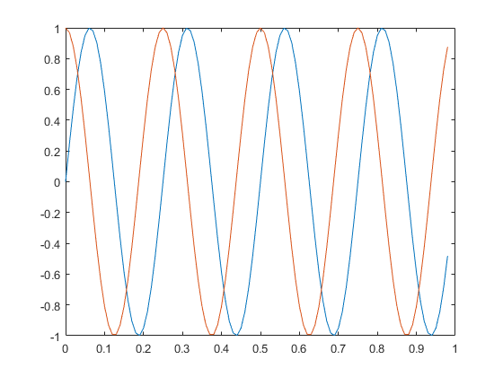
>> t = [0: 0.01: 0.98];
>> y1 = sin(2 * pi * 4 * t);
>> plot(t, y1);
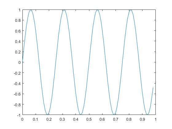
>> y2 = cos(2 * pi * 4 * t);
>> plot(t, y2);
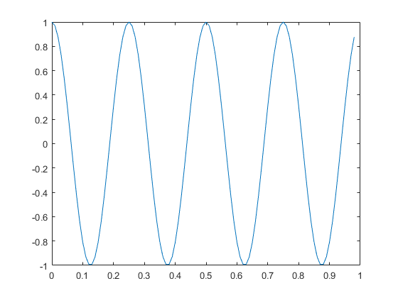
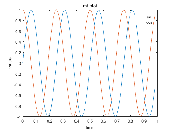
>> plot(t, y1);
>>Hold on;% draw two curves in the same graph
 >>Plot (T, Y2);% plot (T, Y2, 'R') red line
>> xlabel('time')
>> ylabel('value')
>> legend('sin','cos')
>> title('mt plot')
>> print -dpng 'myPlot.png'     %Save to local
>> close     %Close image
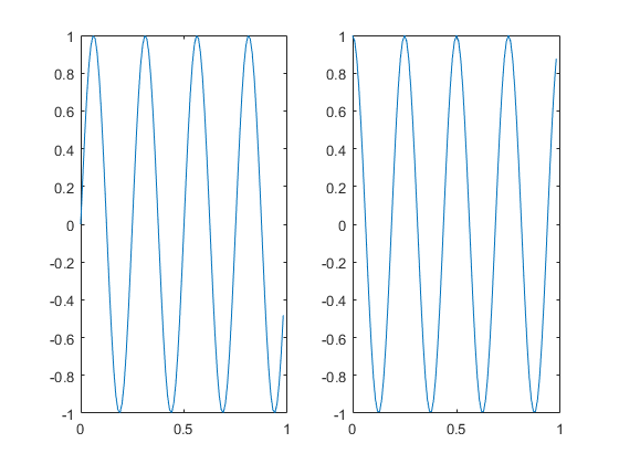
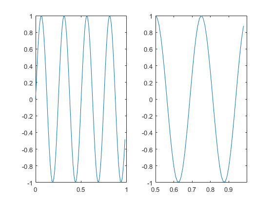
>> figure(1);plot(t, y1);
>> figure(2);plot(t, y2);   %Two images
>>Subplot (1, 2, 1);% divides plot a 1 * 2 grid, access first element
>> plot(t, y1);
>> subplot(1, 2, 2);
>> plot(t, y2);
>>Axis ([0.51-11])% changes x and y axes
>> clf; %Clear an image
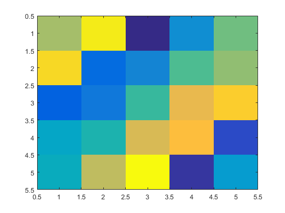
>> A = magic(5)
A =
17 24 1 8 15
23 5 7 14 16
4 6 13 20 22
10 12 19 21 3
11 18 25 2 9
>> imagesc(A) %Visualize a matrix Different colors correspond to different values
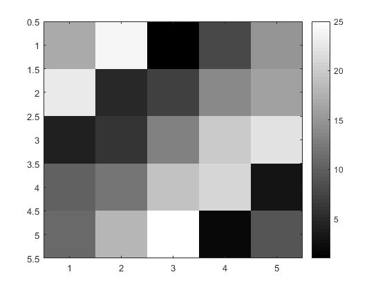
>> imagesc(A), colorbar, colormap gray;
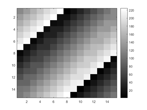
>> imagesc(magic(15)), colorbar, colormap gray;
Control statement
>> v = zeros(10, 1)

v =

     0
     0
     0
     0
     0
     0
     0
     0
     0
     0

>> for i = 1 : 10,    %There's no point in whitespace here, just to make the structure more obvious
       v(i) = 2^i;     % for
   end;
>> v

v =

           2
           4
           8
          16
          32
          64
         128
         256
         512
        1024

>> indices = 1 : 10;
>> indices

indices =

     1     2     3     4     5     6     7     8     9    10

>> for i = indices,
       disp(i);
   end;
     1

     2

     3

     4

     5

     6

     7

     8

     9

    10
>> v

v =

           2
           4
           8
          16
          32
          64
         128
         256
         512
        1024

>> i = 1;
>> while i <= 5,          %while
        v(i) = 100;
        i = i + 1;
  end;
>> v

v =

         100
         100
         100
         100
         100
          64
         128
         256
         512
        1024

>> i = 1;
>> while true,
         v(i) = 999;
         i = i + 1;
         if i == 6,
            break;         %break
         end;
       end;
>> v

v =

         999
         999
         999
         999
         999
          64
         128
         256
         512
        1024
function
>> pwd

ans =

C:\Users\asus\Documents\MATLAB

>> cd 'C:\Users\asus\Desktop'
%Create one on the desktop in advance suqareThisNumber.m Document, open with WordPad is a function

%function y = suqareThisNumber(x)

%y = x^2;

%It is recommended to open the file with WordPad instead of Notepad

>> squareThisNumber(5)

ans =

    25

>> addpath('C:\Users\asus\Desktop')   %Instead of modifying the path, add the path to the search path
>> cd 'C:\'
>> squareThisNumber(5)

ans =

    25

>> pwd

ans =

C:\
>> %Return multiple values
%Create a file on the desktop squareAndCubeThisNumber.m  The contents are as follows
%function [y1, y2] = squareAndCubeThisNumber(x)

%y1 = x^2;
%y2 = x^3;

>> [a, b] = squareAndCubeThisNumber(5);
>> a

a =

    25

>> b

b =

   125
Cost function
%costFunction.m
function J = costFunctionJ(X, y, theta)

%X is the "design matrix" containing our training examples.

%y is the class labels

m = size(X, 1);   %Number of training examples.
predictions = X*theta;    %Predictions of hypothesis on all m examples.
sqrErrors = (predictions - y) .^ 2;    %square errors.

J = 1/(2*m) * sum(sqrErrors);
>> X = [1 1; 1 2; 1 3]

X =

     1     1
     1     2
     1     3

>> y = [1; 2; 3]

y =

     1
     2
     3

>> theta = [0; 1];
>> j = costFunction(X, y, theta)

j =

     0

>> theta = [0; 0];
>> j = costFunction(X, y, theta)

j =

    2.3333
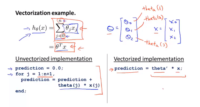
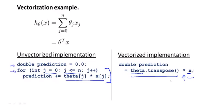
Vectorization