1. Time series algorithm  

1.1 differential autoregressive moving average model (Arima)

1.1.1 overview

         ARIMA is a typical time series model, which consists of three parts: AR model (autoregressive model) and MA model (moving average model), as well as the order I of difference. Therefore, ARIMA is called differential autoregressive moving average model.

reference:

Theoretical sources  

Arima for time series analysis_ CV frontier - CSDN blog_ Basic steps of python time series time series modeling 1. Obtain the time series data of the observed system; 2. Plot the data and observe whether it is a stationary time series; For non-stationary time series, first perform * * d-order difference operation * * to convert it into stationary time series; 3. After the second step, the stationary time series has been obtained. The * * autocorrelation coefficient ACF * * and * * partial autocorrelation coefficient PACF * * of the stationary time series are obtained respectively. Through the analysis of the autocorrelation graph and partial autocorrelation graph, the optimal * * level p * * and * * order q**4 are obtainedhttps://blog.csdn.net/u010414589/article/details/49622625

  Code source

Classic case of time series analysis using ARIMA model (detailed code)_ Xiaobai's coding House - CSDN blog_ The classic case of time series model is because the teacher talked about time series before in the data analysis course, but only briefly introduced this classic time series case, and did not involve the three steps of finding the difference number d, finding the p and q values of ARIMA model and model test. Later, I searched the whole network and finally reorganized the code in combination with the explanations of various articles. The following is the detailed whole code process (if there is a problem, please put forward correction!????): # - * - coding: utf-8 - * -# time series prediction with ARIMAhttps://blog.csdn.net/weixin_41013322/article/details/102710236?ops_request_misc=%257B%2522request%255Fid%2522%253A%2522163832816916780271597143%2522%252C%2522scm%2522%253A%252220140713.130102334..%2522%257D&request_id=163832816916780271597143&biz_id=0&utm_medium=distribute.pc_search_result.none-task-blog-2~all~top_positive~default-1-102710236.first_rank_v2_pc_rank_v29&utm_term=arima&spm=1018.2226.3001.4187

The modified code is as follows:

# -*— coding:utf-8 -*-
# @time   :2021/11/30 15:47
# @Author :zhangzhoubin
# -*- coding: utf-8 -*-
# Time series prediction with ARIMA
import pandas as pd
import numpy as np
import matplotlib.pyplot as plt
import statsmodels.api as sm
from statsmodels.tsa.arima_model import ARIMA
from statsmodels.graphics.tsaplots import acf,pacf,plot_acf,plot_pacf
from statsmodels.graphics.api import qqplot

#Chinese display
plt.rcParams['font.sans-serif']=['SimHei'] #Used to display Chinese labels normally
plt.rcParams['axes.unicode_minus']=False #Used to display negative signs normally

# 1. Create data
data = [5922, 5308, 5546, 5975, 2704, 1767, 4111, 5542, 4726, 5866, 6183, 3199, 1471, 1325, 6618, 6644, 5337, 7064, 2912, 1456, 4705, 4579, 4990, 4331, 4481, 1813, 1258, 4383, 5451, 5169, 5362, 6259, 3743, 2268, 5397, 5821, 6115, 6631, 6474, 4134, 2728, 5753, 7130, 7860, 6991, 7499, 5301, 2808, 6755, 6658, 7644, 6472, 8680, 6366, 5252, 8223, 8181, 10548, 11823, 14640, 9873, 6613, 14415, 13204, 14982, 9690, 10693, 8276, 4519, 7865, 8137, 10022, 7646, 8749, 5246, 4736, 9705, 7501, 9587, 10078, 9732, 6986, 4385, 8451, 9815, 10894, 10287, 9666, 6072, 5418]

data = pd.Series(data)
data.index = pd.Index(sm.tsa.datetools.dates_from_range('1901','1990'))
print(data)
data.plot(figsize=(12,8))
plt.title('Visual display of raw data')
plt.ylabel('Economic growth')
plt.xlabel('particular year')
#Draw the data diagram of timing
plt.show()

#2. Next, we first perform the time series difference on the non-stationary time series to find out the appropriate value of the difference number d:
# fig = plt.figure(figsize=(12, 8))
# ax1 = fig.add_subplot(111)
# diff1 = data.diff(1)
# diff1.plot(ax=ax1)
# plt.title('display of difference results once ')
#The first-order difference is made here. It can be seen that the mean and variance of the time series are basically stable. However, the effect of the second-order difference can be compared:

#The second-order difference is performed here
# fig = plt.figure(figsize=(12, 8))
# ax2 = fig.add_subplot(111)
# diff2 = data.diff(2)
# diff2.plot(ax=ax2)
# plt.title('result display of quadratic difference ')
# plt.show()
#It can be seen from the figure below that the difference between the first-order and the second-order is not very different, so the difference number d can be set to 1. We will comment out the first-order and second-order procedures above

#Here we use the time series of first-order difference
#3. Next, we need to find the appropriate p and q values in ARIMA model:
data1 = data.diff(1)
data1.dropna(inplace=True)
#Add this step, otherwise the acf and pacf diagrams drawn later will be a straight line
#
#Step 1: first check the autocorrelation diagram and partial autocorrelation diagram of stationary series
fig = plt.figure(figsize=(12, 8))
ax1 = fig.add_subplot(211)
fig = sm.graphics.tsa.plot_acf(data1,lags=40,ax=ax1)
#lags represents the order of lag
# #Step 2: acf diagram and pacf diagram are obtained respectively
ax2 = fig.add_subplot(212)
fig = sm.graphics.tsa.plot_pacf(data1, lags=40,ax=ax2)
plt.show()

#As can be seen from the above figure, we can use ARMA(7,0) model, ARMA(7,1) model and ARMA(8,0) model to fit and find the best model:
#Step 3: find out the best model ARMA
arma_mod1 = sm.tsa.ARMA(data1,(7,0)).fit()
print(arma_mod1.aic, arma_mod1.bic, arma_mod1.hqic)
#1580.3025343975862 1602.7002617251756 1589.3304155296435
arma_mod2 = sm.tsa.ARMA(data1,(7,1)).fit()
print(arma_mod2.aic, arma_mod2.bic, arma_mod2.hqic)
#1581.7419537046683 1606.6283174019898 1591.7729327402876
arma_mod3 = sm.tsa.ARMA(data1,(8,0)).fit()
print(arma_mod3.aic, arma_mod3.bic, arma_mod3.hqic)
#1582.027426337836 1606.9137900351575 1592.0584053734553

# #It can be seen from the above that ARMA(7,0) model is the best
# #Step 4: test the model
# #Firstly, the autocorrelation diagram is made for the residual generated by ARMA(7,0) model
# resid = arma_mod1.resid
# #Be sure to add this variable assignment statement, otherwise the error resid is not defined will be reported
# fig = plt.figure(figsize=(12, 8))
# ax1 = fig.add_subplot(211)
# fig = sm.graphics.tsa.plot_acf(resid.values.squeeze(),lags=40,ax=ax1)
# ax2 = fig.add_subplot(212)
# fig = sm.graphics.tsa.plot_pacf(resid, lags=40,ax=ax2)
# #
# #Then do the D-W test
# print(sm.stats.durbin_watson(arma_mod1.resid.values))
# # #The result is that there is no autocorrelation
# #
# # #Then observe whether it conforms to the normal distribution. Here, use the qq diagram
# fig = plt.figure(figsize=(12,8))
# ax = fig.add_subplot(111)
# fig = qqplot(resid, line='q',ax=ax, fit=True)
# plt.show()
# #Finally, Ljung box test is used: the test result is to look at the test probability of the first twelve rows of the last column (generally, the observation lag is 1 ~ 12 orders),
# #If the test probability is less than a given significance level, such as 0.05, 0.10, etc., reject the original hypothesis that the correlation coefficient is zero.
# #From the results, the P values of the first 12 orders are greater than 0.05, so the original assumption is not rejected at the significance level of 0.05, that is, the residual is a white noise sequence.
# r,q,p = sm.tsa.acf(resid.values.squeeze(),qstat=True)
# data2 = np.c_[range(1,41), r[1:], q, p]
# table= pd.DataFrame(data2, columns=[ 'lag','AC','Q','Prob(>Q)'])
# print(table.set_index('lag'))
# #
# #Step 5: forecast the future ten years with the stationary model
# predict_y =arma_mod1.predict('1990', '2000', dynamic=True)
# print(predict_y)   #arima model adopts the calculation method. The number of calculations can be predicted by using the trained model
#
# fig, ax = plt.subplots(figsize=(12,8))
# ax1 = data1.loc['1901':]
# ax = data1.loc['1901':].plot(ax=ax)
# predict_y.plot(ax=ax)
# plt.show()


#Restore to original sequence
ts_restored = pd.Series([data[0]], index=[data.index[0]]) .append(data1).cumsum()   #Since the above difference adopts the difference with the number of steps of 1, the data is restored according to the first data of the original data to obtain the historical original data

#Step 6: use ARIMA model for prediction
model = ARIMA(ts_restored,order=(7,1,0)) #Import ARIMA model
result = model.fit()
predict_y =result.predict('1991', '2000', dynamic=True)
a=pd.concat([data1,predict_y])

#Restore result data + forecast data
res = pd.Series([data[0]], index=[data.index[0]]) .append(a).cumsum()
print(res)  #arima model adopts the calculation method. The number of calculations can be predicted by using the trained model
plt.plot(res,'b')  #Draw the whole curve of real value and predicted value
plt.title('Visualization of real and predicted data (overall rendering)')
plt.show()

#Draw sectional curves of real value and predicted value, and visually analyze the distribution of different predicted values
a=res.loc[:'1990']
b=res.loc['1990':]
plt.plot(a,label="True_valeu",color='b')
plt.plot(b,label="pred_value",color='r',linestyle="--")
plt.title('Visualization of real data and predicted data (piecewise rendering)')
plt.show()

Relevant knowledge supplement

1) Difference

         Difference is a kind of quantization used to reflect the discrete situation of discrete data. It is a tool to study discrete data. The calculation logic is basically consistent with differentiation.

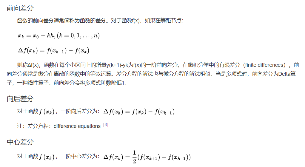
         Difference is also known as difference function or difference operation. The result of difference reflects a change between discrete quantities. It is a tool to study discrete mathematics. It maps the original function f(x) to f(x+a)-f(x+b). Difference operation, corresponding to differential operation, is an important concept in calculus. In a word, difference corresponds to discrete, and differential corresponds to continuous. The difference is divided into forward difference, backward difference and central difference.

         Readers are familiar with the arithmetic sequence: a1   a2   a3... An... Where an+1= an  + D (n = 1,2,... N) d is a constant, called tolerance, i.e. d = an+1  - an  , This is a difference, usually expressed as D(an) = an+1- an, so there is D(an)= d, which is a difference equation in the simplest form.

         Definition. Let the variable y depend on the independent variable T. when t changes to t + 1, the change of dependent variable y = y(t) = y (T + 1) - y(t) is called the (first-order) difference of function y(t) with step size of 1 at point t, which is recorded as Dy1= yt+1- yt, which is referred to as the (first-order) difference of function y(t), and D is called the difference operator.  

Difference has operational properties similar to differential.