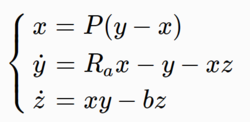
Lorenz equation is a simplified differential equation system describing the motion of air fluid. In 1963, American meteorologist Lorenz (E. N.) will boldly truncate a set of non-linear partial differential equations describing atmospheric heat convection and derive a three-dimensional autonomous dynamic system describing vertical velocity and temperature difference by means of Fourier expansion.

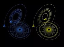
P: Prandt number and Ra Rayleigh number. He found that when Ra increased, the system bifurcated from the stationary state to the periodic state (convective state). Finally, when Ra > 24.74, the non-periodic chaotic state (turbulent state). As shown in the figure, the chaotic state in the three-dimensional phase space projected onto the two-dimensional plane. From the graph, the trajectory was initially from the right side. Outward and inward circle, then randomly jump to the left and outward and inward circle, and then again randomly jump back to the right circle,... As Lorentz is the first person in the world to discover the non-periodic chaos phenomenon from a definite equation, the above equation is generally called Lorentz equation.

#!/usr/bin/python
# -*- coding:utf-8 -*-

from scipy.integrate import odeint
import numpy as np
import matplotlib as mpl
import matplotlib.pyplot as plt
from mpl_toolkits.mplot3d import Axes3D


def lorenz(state, t):
    # print w
    # print t
    sigma = 10
    rho = 28
    beta = 3
    x, y, z = state
    return np.array([sigma*(y-x), x*(rho-z)-y, x*y-beta*z])


def lorenz_trajectory(s0, N):
    sigma = 10
    rho = 28
    beta = 8/3.

    delta = 0.001
    s = np.empty((N+1, 3))
    s[0] = s0
    for i in np.arange(1, N+1):
        x, y, z = s[i-1]
        a = np.array([sigma*(y-x), x*(rho-z)-y, x*y-beta*z])
        s[i] = s[i-1] + a * delta
    return s


if __name__ == "__main__":
    mpl.rcParams['font.sans-serif'] = ['SimHei']
    mpl.rcParams['axes.unicode_minus'] = False

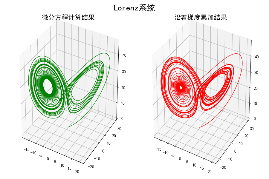
    # Figure 1
    s0 = (0., 1., 0.)
    t = np.arange(0, 30, 0.01)
    s = odeint(lorenz, s0, t)
    plt.figure(figsize=(9, 6), facecolor='w')
    plt.subplot(121, projection='3d')
    plt.plot(s[:, 0], s[:, 1], s[:, 2], c='g', lw=1)
    plt.title('Calculations of Differential Equations', fontsize=16)

    s = lorenz_trajectory(s0, 40000)
    plt.subplot(122, projection='3d')
    plt.plot(s[:, 0], s[:, 1], s[:, 2], c='r', lw=1)
    plt.title('Cumulative results along the gradient', fontsize=16)

    plt.tight_layout(1, rect=(0,0,1,0.98))
    plt.suptitle('Lorenz system', fontsize=20)
    plt.show()

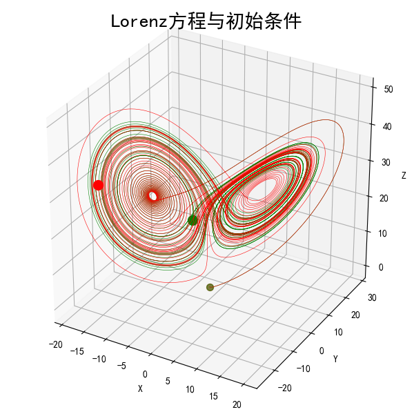
    # Figure 2
    ax = Axes3D(plt.figure(figsize=(6, 6)))
    s0 = (0., 1., 0.)
    s1 = lorenz_trajectory(s0, 50000)
    s0 = (0., 1.0001, 0.)
    s2 = lorenz_trajectory(s0, 50000)
    # curve
    ax.plot(s1[:, 0], s1[:, 1], s1[:, 2], c='g', lw=0.4)
    ax.plot(s2[:, 0], s2[:, 1], s2[:, 2], c='r', lw=0.4)
    # Starting point
    ax.scatter(s1[0, 0], s1[0, 1], s1[0, 2], c='g', s=50, alpha=0.5)
    ax.scatter(s2[0, 0], s2[0, 1], s2[0, 2], c='r', s=50, alpha=0.5)
    # End
    ax.scatter(s1[-1, 0], s1[-1, 1], s1[-1, 2], c='g', s=100)
    ax.scatter(s2[-1, 0], s2[-1, 1], s2[-1, 2], c='r', s=100)
    ax.set_title('Lorenz Equations and Initial Conditions', fontsize=20)
    ax.set_xlabel('X')
    ax.set_ylabel('Y')
    ax.set_zlabel('Z')
    plt.show()