When learning machine learning, many students start programming directly after a rough look at the theory, which is very commendable. However, it's not really a handwriting algorithm, but to directly call a package such as sklearn, which is not appropriate. The author is not saying that the package transfer is bad. In practical work and research, the encapsulated and easy-to-use package has brought great convenience to our work and greatly improved the implementation efficiency of our machine learning model and algorithm. However, this is limited to the use process.

     I believe that many ambitious students are certainly not satisfied with using these packages without knowing the details of models and algorithms. Therefore, if you are a learner of machine learning algorithm, you'd better not use these encapsulated packages as soon as you come up in the learning process. Instead, according to your own understanding of the algorithm, after pushing the mathematical formula of the model and algorithm by hand, you can only rely on basic packages such as numpy and pandas to write the machine learning algorithm. After this process, learn how to call sklearn and other machine learning libraries. I believe you can better experience the convenience and fun of packet switching. After that, go to data practice and play games. I believe you will become an excellent machine learning algorithm engineer.

     The two topics of this machine learning series are mathematical derivation + pure numpy implementation. Let's start with the most basic linear regression model. I believe you must be quite familiar with the regression algorithm, especially our students with statistical background. Therefore, the author makes a direct mathematical derivation.

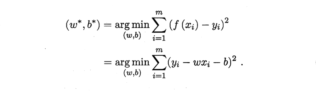
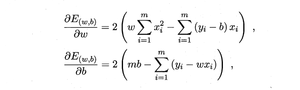
Mathematical derivation of regression analysis

     Originally, I wanted to use the author's hand push draft, but the handwriting is too publicized, and writing formulas in word or markdown is too time-consuming. Here, I directly borrow the derivation process in teacher Zhou Zhihua's machine learning textbook:

 

     Extended to matrix form:

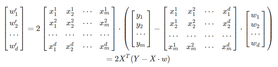
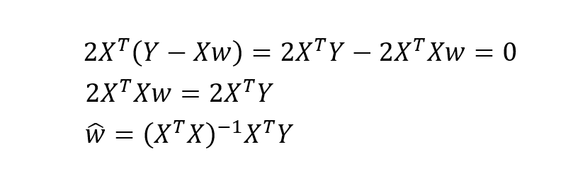
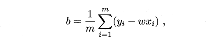
     The above is the derivation process of parameter estimation in linear regression model.

numpy implementation of regression analysis

     According to the Convention, we need to sort out the writing ideas before writing the algorithm. The main part of the regression model is relatively simple. The key is how to update the parameters based on gradient descent after giving the mse loss function. Firstly, we need to write the main body of the model, the loss function and the parameter derivation results based on the loss function, then initialize the parameters, and finally write the parameter update process based on the gradient descent method. Of course, we can also write cross validation to get more robust parameter estimates. Don't say much, just go to the code.

     Regression model body:

import numpy as np

def linear_loss(X, y, w, b):    
    num_train = X.shape[0]    
    num_feature = X.shape[1]    
    # Model formula    
    y_hat = np.dot(X, w) + b    
    # Loss function   
    loss = np.sum((y_hat-y)**2)/num_train    
    # Partial derivative of parameters    
    dw = np.dot(X.T, (y_hat-y)) /num_train    
    db = np.sum((y_hat-y)) /num_train    
    return y_hat, loss, dw, db

 

Parameter initialization:

def initialize_params(dims):    
    w = np.zeros((dims, 1))   
    b = 0    
    return w, b

     Model training process based on gradient descent:

def linar_train(X, y, learning_rate, epochs):    
    w, b = initialize(X.shape[1])  
    loss_list = []  
    for i in range(1, epochs):        
    # Calculate the current predicted value, loss and parameter partial derivative        
        y_hat, loss, dw, db = linar_loss(X, y, w, b)  
        loss_list.append(loss)      
        # Parameter updating process based on gradient descent        
        w += -learning_rate * dw        
        b += -learning_rate * db        
        # Print iterations and losses        
        if i % 10000 == 0:            
            print('epoch %d loss %f' % (i, loss))
              
       # Save parameters        
        params = {            
           'w': w,            
           'b': b        
        }        
       
       # Save gradient        
        grads = {            
           'dw': dw,            
           'db': db        
        }    
           
    return loss_list, loss, params, grads

     The above is the basic implementation process of linear regression model. Let's take the diabetes dataset in sklearn as an example for simple training.

     Data preparation:

from sklearn.datasets import load_diabetes
from sklearn.utils import shuffle
 
diabetes = load_diabetes() 
data = diabetes.data 
target = diabetes.target 

# Scramble data
X, y = shuffle(data, target, random_state=13) 
X = X.astype(np.float32)

# Simple division of training set and test set
offset = int(X.shape[0] * 0.9) 
X_train, y_train = X[:offset], y[:offset] 
X_test, y_test = X[offset:], y[offset:] 
y_train = y_train.reshape((-1,1)) 
y_test = y_test.reshape((-1,1))
 
print('X_train=', X_train.shape) 
print('X_test=', X_test.shape) 
print('y_train=', y_train.shape) 
print('y_test=', y_test.shape)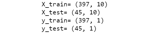

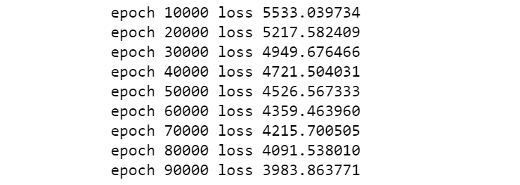
     Perform training:

loss_list, loss, params, grads = linar_train(X_train, y_train, 0.001, 100000)

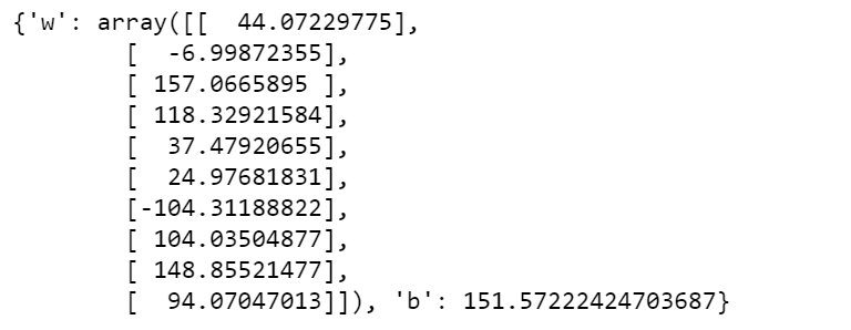
     View the regression model parameter values obtained from training:

print(params)

     The following defines a prediction function to predict the test set results:

def predict(X, params):   
    w = params['w']    
    b = params['b']    

    y_pred = np.dot(X, w) + b    
    return y_pred 

y_pred = predict(X_test, params) 
y_pred[:5]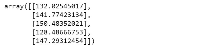

     Use matplotlib to display the prediction results and true values:

import matplotlib.pyplot as plt 
f = X_test.dot(params['w']) + params['b'] 

plt.scatter(range(X_test.shape[0]), y_test) 
plt.plot(f, color = 'darkorange') 
plt.xlabel('X') 
plt.ylabel('y') 
plt.show()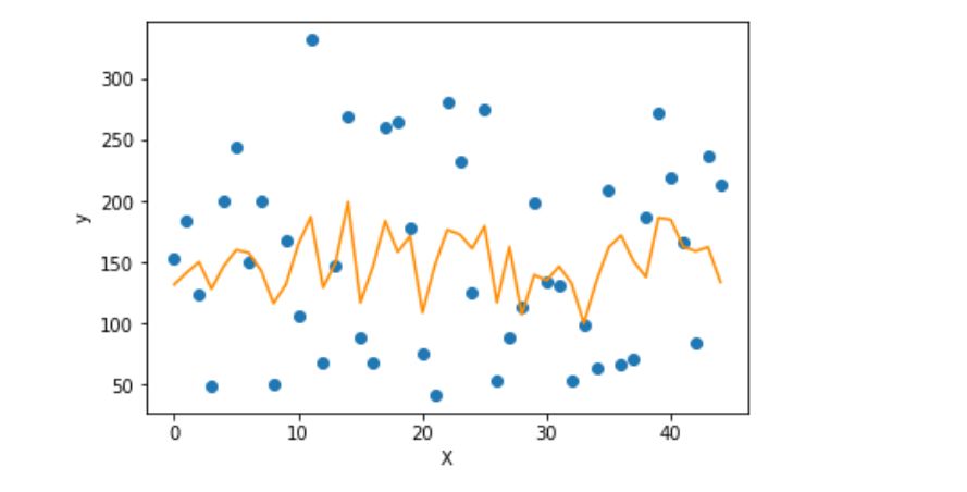

     It can be seen that the data of all variables is not good for the fitting and combination of linear regression model. First, the distribution of the data itself, and second, the fitting effect of simple linear model is poor for the data. Of course, we just want to demonstrate the basic process of linear regression model, and don't care about the effect.

     Loss reduction during training:

plt.plot(loss_list, color = 'blue') 
plt.xlabel('epochs') 
plt.ylabel('loss') 
plt.show()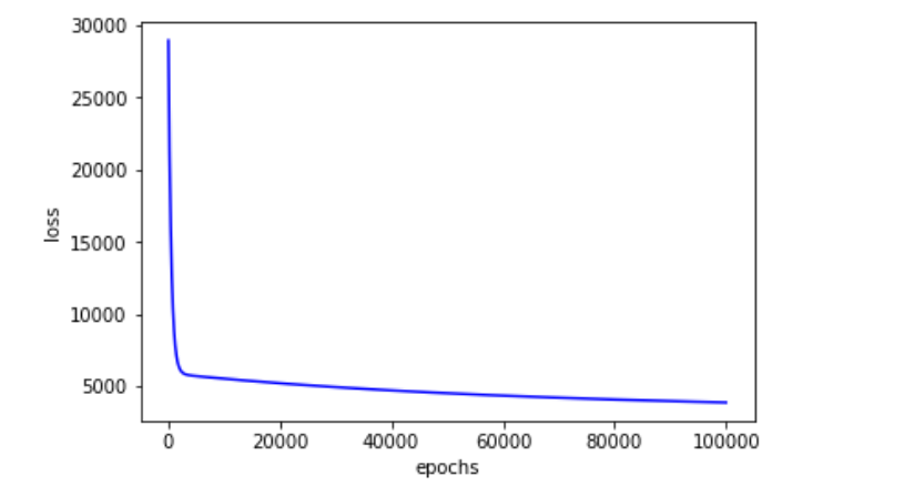

Encapsulate a linear regression class

     The author makes a simple class encapsulation for the above process, in which a user-defined cross validation process is added for training:

import numpy as np
from sklearn.utils import shuffle
from sklearn.datasets import load_diabetes

class lr_model():    
    def __init__(self):        
        pass    

    def prepare_data(self):        
        data = load_diabetes().data        
        target = load_diabetes().target        
        X, y = shuffle(data, target, random_state=42)        
        X = X.astype(np.float32)            
        y = y.reshape((-1, 1))        
        data = np.concatenate((X, y), axis=1)        
        return data  
        
    def initialize_params(self, dims):        
        w = np.zeros((dims, 1))        
        b = 0        
        return w, b    
   
    def linear_loss(self, X, y, w, b):        
        num_train = X.shape[0]        
        num_feature = X.shape[1]
        
        y_hat = np.dot(X, w) + b        
        loss = np.sum((y_hat-y)**2) / num_train        
        dw = np.dot(X.T, (y_hat - y)) / num_train        
        db = np.sum((y_hat - y)) / num_train        
        return y_hat, loss, dw, db    
   
    def linear_train(self, X, y, learning_rate, epochs):        
        w, b = self.initialize_params(X.shape[1])        
        for i in range(1, epochs):            
            y_hat, loss, dw, db = self.linear_loss(X, y, w, b)            
            w += -learning_rate * dw                
            b += -learning_rate * db                
            if i % 10000 == 0:                
                print('epoch %d loss %f' % (i, loss))
            params = {                
               'w': w,                
               'b': b            
            }            
            grads = {                
               'dw': dw,                
               'db': db            
            }        
        return loss, params, grads    
   
    def predict(self, X, params):        
        w = params['w']        
        b = params['b']        
        y_pred = np.dot(X, w) + b        
        return y_pred    
       
    def linear_cross_validation(self, data, k, randomize=True):        
        if randomize:            
            data = list(data)            
            shuffle(data)
        
        slices = [data[i::k] for i in range(k)]        
        for i in range(k):            
            validation = slices[i]            
            train = [data                        
            for s in slices if s is not validation for data in s]            
            train = np.array(train)            
            validation = np.array(validation)            
            yield train, validation
           
           
if __name__ == '__main__':    
    lr = lr_model()    
    data = lr.prepare_data()
  
    for train, validation in lr.linear_cross_validation(data, 5):        
        X_train = train[:, :10]        
        y_train = train[:, -1].reshape((-1, 1))        
        X_valid = validation[:, :10]        
        y_valid = validation[:, -1].reshape((-1, 1))        

        loss5 = []        
        loss, params, grads = lr.linear_train(X_train, y_train, 0.001, 100000)
        loss5.append(loss)        
        score = np.mean(loss5)        
        print('five kold cross validation score is', score)        
        y_pred = lr.predict(X_valid, params)        
        valid_score = np.sum(((y_pred - y_valid) ** 2)) / len(X_valid)
        print('valid score is', valid_score)

The above is the content of this section. A simple linear regression model is manually implemented based on numpy.