2.1 linear regression algorithm model representation
Let's start with an example: this example is to predict housing prices. We want to use a data set containing housing prices in Portland, Oregon. Here, I want to draw my data set according to the selling prices of different house sizes. For example, if your friend's house is 1250 square feet, you should tell them how much the house can sell. Well, one thing you can do is build a model, maybe a straight line. From this data model, maybe you can tell your friend that he can sell the house for about 220000 dollars. This is an example of a supervised learning algorithm.
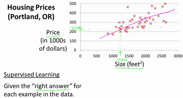
It is called supervised learning because for each data, we give the "correct answer", that is, tell us: according to our data, what is the actual price of the house, which is a regression problem. Regression means that we predict an accurate output value based on previous data. For this example, price. At the same time, there is another most common supervised learning method, called classification problem. When we want to predict discrete output values, for example, we are looking for cancer and want to determine whether the tumor is benign or malignant, This is the problem of 0 / 1 discrete output.
Furthermore, in supervised learning, we have a data set, which is called training set.
I will use lowercase throughout the course to represent the number of training samples.
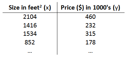
Taking the previous housing transaction problem as an example, suppose we return to the Training Set of the problem as shown in the following table:
The markers we will use to describe this regression problem are as follows:
m represents the number of instances in the training set
x stands for characteristic / input variable
y represents the target variable / output variable
(x,y) represents an instance of the training set
(x(i),y(i)) represents the ith observation example
h represents the solution or function of the learning algorithm, also known as hypothesis
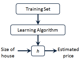
The working mode of supervised learning algorithm can output one by introducing the training set in the data set into the linear model algorithm
We can see here the house price in our training set. We feed it to our learning algorithm. The learning algorithm works, and then output a function, usually expressed as lowercase H. It stands for hypothesis (hypothesis) and represents a function. The input is the size of the house, just like the house your friend wants to sell. Therefore, H obtains the y value according to the input x value, and the y value corresponds to the price of the house. Therefore, h is a function mapping from X to y.
I will choose the initial use rule to represent hypothesis. Therefore, to solve the problem of house price prediction, we actually "feed" the training set to our learning algorithm, and then learn to get a hypothesis, and then input the size of the house we want to predict as an input variable to, predict the transaction price of the house as an output variable, and output as a result. So, how should we express our house price forecast ?
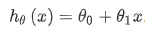
One possible expression is:
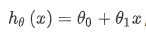
Because there is only one characteristic / input variable, such a problem is called univariate linear regression problem.
2.2 cost function
The concept of cost function is helpful to understand how to fit the most likely straight line with the data.
As shown in the figure:
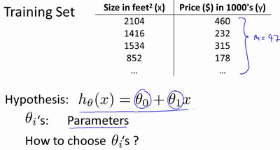
In linear regression, we have a training set like this, which represents the number of training samples, such as m=47. Our hypothetical function, that is, the function used for prediction, is in the form of linear function:
Next, we will introduce some terms. What we need to do now is to select the appropriate parameters for our model θ 0 and θ one , In the case of house price problem, it is the slope of the straight line and the intercept on the y-axis.
The parameters we choose determine the accuracy of the straight line we get relative to our training set. The difference between the predicted value of the model and the actual value in the training set (referred to by the blue line in the figure below) is the modeling error.
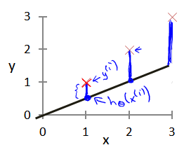
Our goal is to select the model parameters that can minimize the sum of squares of modeling errors. Even if the cost function minimum.
We draw a contour map with three coordinates of and And:
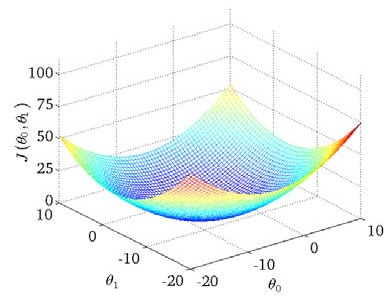
It can be seen that there is a minimum point in three-dimensional space.
The cost function is also called the square error function, sometimes called the square error cost function. The reason why we require the sum of squares of errors is that the square cost function of errors is a reasonable choice for most problems, especially regression problems. There are other cost functions that can also play a good role, but the square error cost function may be the most commonly used means to solve the regression problem.
Through the exhaustive method to find the lowest point or the minimum error
Data set design
Problem: as shown in Figure 1, the value x of the time y and final score invested by students in A course every week, so set y=wx, and design an algorithm to find the best fitting value of the weight of w.
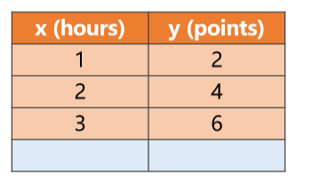 Figure 1 data set
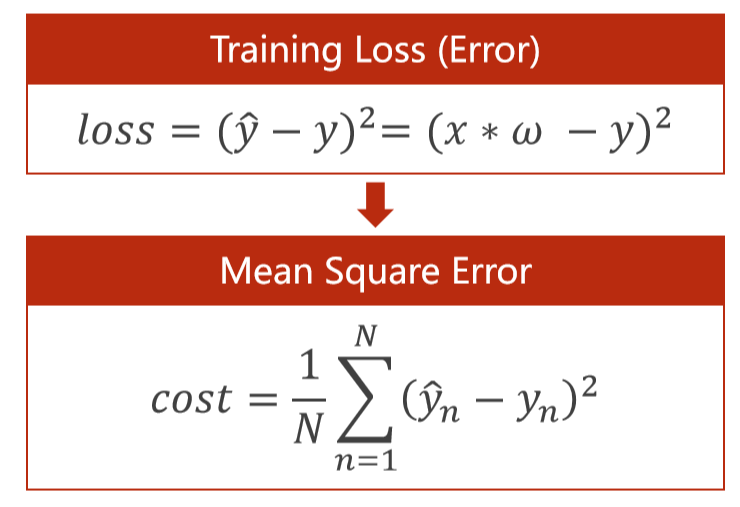 Figure 2 loss function
code:
import numpy as np
import matplotlib.pyplot as plt
#data set
x_data=[1.0,2.0,3.0]
y_data=[2.0,4.0,6.0]
#Build y = w * x = = > predicted value
def forward(x):
return x*w
#Calculate loss, i.e. the loss formula is shown in the figure above, and the error is calculated by subtracting the original data from the predicted value
def loss(x,y):
y_pred=forward(x)
return (y_pred-y)*(y_pred-y)
#List of weights w
w_list=[]
#List of loss
mse_list=[]
#The best fitting value of y=w*x is calculated by using the exhaustive method for W
for w in np.arange(0.0,4.1,0.1):
print(w)
l_sum=0
#zip() when the length of the passed parameters is different, the shorter one is used as the standard
for x_val,y_val in zip(x_data,y_data):
#Calculate new forecast
y_pred_val=forward(x_val)
#New forecasts and
loss_val=loss(x_val,y_val)
l_sum= l_sum+loss_val
print(x_val,y_val,y_pred_val,loss_val)
#Divided by the number of samples, i.e. the average error
MSR=l_sum/3
w_list.append(w)
mse_list.append(MSR)
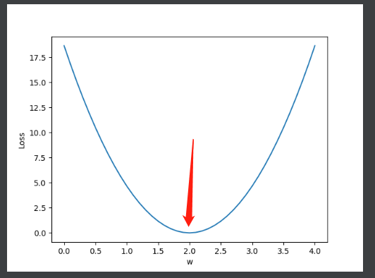
#Draw the function image between loss and weight w
plt.plot(w_list,mse_list)
plt.ylabel('Loss')
plt.xlabel('w')
plt.show()
Operation results: it can be seen that when w is 2, the loss of loss is the smallest
Question 2
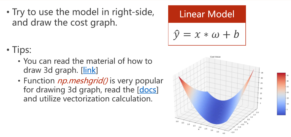
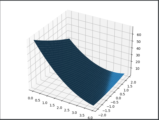
Homework topic: realize the linear model (y=wx+b) and output the 3D image of loss.
import numpy as np
import matplotlib.pyplot as plt
from mpl_toolkits.mplot3d import Axes3D

#data set
x_data = [1.0,2.0,3.0]
y_data = [5.0,8.0,11.0]

# Data set length
m=len(x_data)

# Weight
W=np.arange(0.0,4.0,0.1)
B=np.arange(-2.0,2.0,0.1)
[w,b]=np.meshgrid(W,B)
#That is, in three-dimensional coordinates, W is X week and B is Y week. You must use lowercase when drawing, because lowercase is n × N is a two-dimensional array, in uppercase, an array composed of one-dimensional n numbers

# Pay attention to the operation of the matrix
def farword(x):
    return x * w+b

def loss(y_test,y):
    return (y_test-y)*(y_test-y)

total_loss = 0
for x_val,y_val in zip(x_data,y_data):
    y_test=farword(x_val)
    total_loss=(total_loss+loss(y_test,y_val))/m

fig = plt.figure()

# MatplotlibDeprecationWarning: Calling gca() with keyword arguments was deprecated in Matplotlib 3.4. Starting two minor releases later, gca() will take no keyword arguments. The gca() function should only be used to get the current axes, or if no axes exist, create new axes with default keyword arguments. To create a new axes with non-default arguments, use plt.axes() or plt.subplot().
# ax = fig.gca(projection='3d ') is changed to
# ax = fig.add_subplot(projection='3d')
ax = Axes3D(fig)

print(W.shape) #(40,)
print(W)
print(w.shape)#(40,40)
print(w)

# ax.plot_surface(W,B,total_loss)
ax.plot_surface(w,b,total_loss)
plt.show()
design sketch
numpy.meshgrid() understand
 https://blog.csdn.net/lllxxq141592654/article/details/81532855