least square method

1. What is the essence of least squares
   Taking measuring the length with different rulers as an example, several measured values are obtained. How to determine the true value? "y, which minimizes the sum of squares of errors, is the true value." this is based on the fact that if the error is random, the measured value will fluctuate up and down the true value. Ruler example, optimization goal m i n ∑ ( y − y i ) 2 min \sum(y-y_i)^2 min Σ (Y − yi) 2, then the objective function takes the derivative of Y, and y with zero derivative is exactly the arithmetic mean. Least square -- > least + square
2. Generalization: for polynomial fitting
3. MATLAB implementation
   3.1 solving equations
   Least squares principle and MATLAB code - linear fitting, polynomial fitting and specified function fitting
   3.1.1 linear equation
   m i n ∑ ( y i − a x i − b ) 2 = 0 min \sum(y_i-ax_i-b)^2=0 min Σ (yi − axi − b)2=0, calculate the partial derivatives of a and B as 0 respectively, and obtain the following equations to solve a and B. In addition, the equations can be written in matrix form.
   { − ∑ 2 ( y i − a x i − b ) x i = 0 − ∑ 2 ( y i − a x i − b ) = 0 \left\{ \begin{array}{c} -\sum{2\left( y_i-ax_i-b \right) x_i=0}\\ -\sum{2\left( y_i-ax_i-b \right) =0} \end{array} \right. {−∑2(yi​−axi​−b)xi​=0−∑2(yi​−axi​−b)=0​ ( ∑ 1 ∑ x i ∑ x i ∑ x i 2 ) ( b a ) = ( ∑ y i ∑ y i x i ) \left( \begin{array}{c} \begin{matrix} \sum{1}& \sum{x_i}\\ \end{matrix}\\ \begin{matrix} \sum{x_i}& \sum{x_{i}^{2}}\\ \end{matrix}\\ \end{array} \right) \left( \begin{array}{c} b\\ a\\ \end{array} \right) =\left( \begin{array}{c} \sum{y_i}\\ \sum{y_ix_i} \end{array} \right) (∑ 1 ∑ xi ∑ xi ∑ xi2) (ba) = (∑ yi ∑ yi xi) 3.1.2 polynomial, which can also be written in matrix form similar to the above. XA=Y, then A=inv(X)*Y
   3.2 the optimization problem can be solved by gradient descent method. But the following code does not optimize the step size, which takes time.

clear;
clf;
x0 = linspace(-1,1,100);
% function+Noise
y0 = sin(2*x0).*((x0.^2-1).^3+1/2)+(0.2*rand(1,100)-0.1);
% Raw data image
plot(x0,y0,'.');
% Fitting with polynomial function f(x)
% f(x)=a0+a1*x+...+ak*x^k
% Objective function: sum of squares of errors sum(y-f(x))^2
% Find the optimal value: the partial derivative of each coefficient is 0
% Method 1: solving linear equations XA=Y，be A=Y/X
% Method 2: gradient descent method
% Specify polynomial coefficients k
order = 10;
ini_A = zeros(1,order+1);  % Initial point
% The objective function is to minimize the sum of squares of errors, the initial point is given, and the gradient descent method is used to find the optimal solution
[A,k,err_ols] = GradientMethod_ols(x0, y0, order, ini_A);
y1 = polyfun(x0,order,A);
hold on;
plot(x0,y1);

function [A,k,err_ols] = GradientMethod_ols(x0, y0, order, ini_A)
% x,y: Raw data point
% order,ini_A: A polynomial function is determined
%% Step 1: give the initial iteration point A，Convergence accuracy err，k=1
k = 1;
iterk = 1000;
A = ini_A;
err = 0.5;
%% Step 2:Calculate the gradient and modulus and take the search direction
err_ols = 100;
while(k<iterk)
    grad = gradofpolyols(x0,y0,order,A);
    dir = -grad;  % The search direction is a negative gradient direction
    %% Step 3:Make convergence judgment
    if err_ols<=err  % The gradient is equal to 0
        disp('The error is small enough');
        break;
    end
%% The fourth step is to find the optimal step size and new iteration points 
    lmd_opt = 0.1;  % Take the fixed value directly
    A0 = A;
    while(1)   
    A = A0 + dir*lmd_opt;
    err_ols_1 = sum((y0-polyfun(x0,order,A)).^2);
    if err_ols_1<err_ols
        err_ols = err_ols_1;
        break
    end
    lmd_opt = lmd_opt*0.5;    
    end
    k = k+1;
end
if k >=iterk
disp('The number of iterations has reached the upper limit!');
end
end

function grad = gradofpolyols(x0,y0,order,A)
% Find gradient
grad = zeros(1,length(A));
for i = 1:length(A)
    grad(i) = -2*(y0-polyfun(x0,order,A))*(x0.^(i-1))';
end
end

function y = polyfun(x,order,A)
% Value of polynomial function
% y=a0+a1*x+...+ak*x^k
% x independent variable
% k Polynomial order
% A Coefficient vector
y = zeros(1,length(x));
for i =0:order
    y = y + A(i+1)*x.^i;
end
end

1. supplement
   Line fitting (W=inv(A '* A)*A' * Y / / w = inv (R) * q '* Y) and lsqcurvefit function
   Least square method of MATLAB
   b.

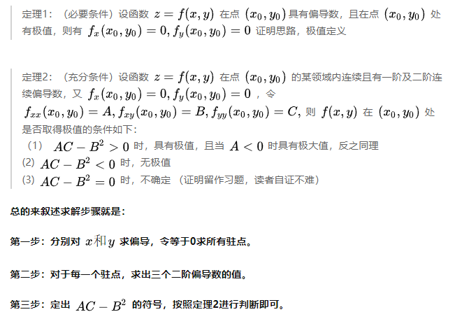
Finding the extreme point of multivariate function

I've forgotten that the extreme value of a multivariate function is the partial derivative of each item, so review it.
1. The point where the first derivative is 0 is called the stagnation point, which is not necessarily the extreme point( y = x 3 y=x^3 y=x3), the extreme point is not necessarily the stationary point( y = ∣ x ∣ y=|x| y=∣x∣)； For multivariate functions, stationary points are all points where the first derivative is zero.
2. The point where the curve convexity changes is the inflection point. If the function is second-order continuous differentiable, the inflection point can deduce that the second-order derivative is 0;
3. The extreme point is the abscissa of the upper maximum or minimum point in a certain sub interval of the function image, which appears at the stationary point or non differentiable point.
Extremum of multivariate function and its solution
( f ( x ) = x 2 , f ′ ′ ( x ) 2 = 4 > 0 , f ′ ′ ( x ) = 2 > 0 have extremely Small value F (x) = x ^ 2, f '' (x) ^ 2 = 4 > 0, f '' (x) = 2 > 0 has a minimum f(x)=x2,f ′′′ (x) 2 = 4 > 0, f ′′ (x) = 2 > 0 (with minimum)
If the known function has and has only one extreme point, then "find the point with partial derivative of 0 to get the extreme point", is that right?