Article directory
- 1. Master the NumPy array object ndarray
- 1.1. Array attribute: ndarray (array) is a multidimensional array that stores a single data type.
- 1.2 array creation
- 1.2.1 reset shape attribute of array
- 1.2.2 create an array using the range function
- 1.2.3 using linspace function to create array -- equal difference
- 1.2.4 using logspace function to create sequence - equal ratio
- 1.2.5 create array with zeros function -- all "0"
- 1.2.6 create array with ones function -- all "1"
- 1.2.7 use eye function to create array -- diagonal is "1"
- 1.2.8 use diag function to create array -- diagonal is the specified content
- 1.3. Array data type
- 2. Generate random number
- 2.1 generating random numbers without constraints
- 2.2. Generate random numbers subject to uniform distribution
- 2.3. Generating random numbers subject to normal distribution
- 2.4 generate random number with given upper and lower range
- 3. Accessing arrays by index
- 4. Transform the shape of an array
1. Master the NumPy array object ndarray
1.1. Array attribute: ndarray (array) is a multidimensional array that stores a single data type.
| attribute | Explain |
|---|---|
| ndim | Returns int. Represents the dimension of an array |
| shape | Return to tuple. Represents the size of the array. For the matrix with n rows and m columns, the shape is (n,m) |
| size | Returns int. Represents the total number of elements in an array, equal to the product of the array shape |
| dtype | Returns data type. Describes the type of elements in an array |
| itemsize | Returns int. Represents the size (in bytes) of each element of the array |
1.2 array creation
numpy.array(object, dtype=None, copy=True, order='K',subok=False, ndmin=0)
| Parameter name | Explain |
|---|---|
| object | Receive array. Represents the array you want to create. No default. |
| dtype | Receive data type. Represents the data type required by the array. If not given, select the minimum type required to save the object. The default is None. |
| ndmin | Receive int. Specifies the minimum dimension that the generated array should have. The default is None. |
(1) Create a one-dimensional array
import numpy as np
np.array([1,2,3])#This is a one-dimensional array
Result:
array([1, 2, 3])
import numpy as np
a = np.array([1,2,3])#This is a one-dimensional array
a.size#The result is 3
a.shape#The result is (3,)
(2) Create a 2D array
import numpy as np
np.array([[1,2,3],[1,2,4]])#This is a two-dimensional array
array([[1, 2, 3],
       [1, 2, 4]])
- View related information
import numpy as np
a = np.array([[1,2,3],[1,2,4]])#This is a two-dimensional array

a.size #The result is 6
a.ndim #Dimension result is 2
a.shape #2 rows and 3 columns (2,3)

a.dtype
dtype('int32')
(3) Forced conversion type
a = np.array([[1,2,3],[1,2,4]],dtype=np.float32)#This is a two-dimensional array
a.dtype
Result:
dtype('float32')
1.2.1 reset shape attribute of array
- Change the data of the above two rows and three columns to three rows and two columns
a.reshape(3,2)
Result:
array([[1., 2.],
       [3., 1.],
       [2., 4.]], dtype=float32)
1.2.2 create an array using the range function
list(range(10))
[0, 1, 2, 3, 4, 5, 6, 7, 8, 9]
np.arange(10)
array([0, 1, 2, 3, 4, 5, 6, 7, 8, 9])
1.2.3 using linspace function to create array -- equal difference
np.linspace( start, stop,num=50, endpoint=True, retstep=False, dtype=None, axis=0)
- num defaults to 50
np.linspace(0,10)#0 ~ 1, 50 by default
Result:
array([ 0.        ,  0.20408163,  0.40816327,  0.6122449 ,  0.81632653,
        1.02040816,  1.2244898 ,  1.42857143,  1.63265306,  1.83673469,
        2.04081633,  2.24489796,  2.44897959,  2.65306122,  2.85714286,
        3.06122449,  3.26530612,  3.46938776,  3.67346939,  3.87755102,
        4.08163265,  4.28571429,  4.48979592,  4.69387755,  4.89795918,
        5.10204082,  5.30612245,  5.51020408,  5.71428571,  5.91836735,
        6.12244898,  6.32653061,  6.53061224,  6.73469388,  6.93877551,
        7.14285714,  7.34693878,  7.55102041,  7.75510204,  7.95918367,
        8.16326531,  8.36734694,  8.57142857,  8.7755102 ,  8.97959184,
        9.18367347,  9.3877551 ,  9.59183673,  9.79591837, 10.        ])
- Restricted number
np.linspace(0,10,10)#Limit 10
array([ 0.        ,  1.11111111,  2.22222222,  3.33333333,  4.44444444,
        5.55555556,  6.66666667,  7.77777778,  8.88888889, 10.        ])
- Limit end value:
np.linspace(0,10,10,endpoint=False)#From 0 to 9, excluding 10
Equivalent to
np.linspace(0,9,10)#Limit 10
array([0., 1., 2., 3., 4., 5., 6., 7., 8., 9.])
1.2.4 using logspace function to create sequence - equal ratio
np.logspace( start, stop, num=50, endpoint=True, base=10.0, dtype=None, axis=0 )
- Default common ratio is 10
np.logspace(0,10,10,endpoint=False)#base is common ratio 10
array([1.e+00, 1.e+01, 1.e+02, 1.e+03, 1.e+04, 1.e+05, 1.e+06, 1.e+07,
       1.e+08, 1.e+09])
- Equal to the 10th power of the last sequence of equal difference numbers
10**np.linspace(0,10,10,endpoint=False)
array([1.e+00, 1.e+01, 1.e+02, 1.e+03, 1.e+04, 1.e+05, 1.e+06, 1.e+07,
       1.e+08, 1.e+09])
- Set common ratio to 2
np.logspace(0,10,10,endpoint=False,base=2)#The common ratio is 2.
array([ 1., 2., 4., 8., 16., 32., 64., 128., 256., 512.])
1.2.5 create array with zeros function -- all "0"
- 1 rows and 2 columns
np.zeros((2))
array([0., 0.])
- 2 rows and 3 columns
np.zeros((2,3))#2 rows and 3 columns
array([[0., 0., 0.],
       [0., 0., 0.]])
1.2.6 create array with ones function -- all "1"
- 1 rows and 3 columns
np.ones((3))
array([1., 1., 1.])
- 3 rows and 5 columns
np.ones((3,5))
array([[1., 1., 1., 1., 1.],
       [1., 1., 1., 1., 1.],
       [1., 1., 1., 1., 1.]])
1.2.7. Use the eye function to create an array -- the diagonal line is "1"
- 1 rows and 3 columns
np.eye((3))
array([[1., 0., 0.],
       [0., 1., 0.],
       [0., 0., 1.]])
1.2.8 use diag function to create array -- diagonal is the specified content
- 1, 2, 3, 4 diagonal
np.diag((1,2,3,4))
array([[1, 0, 0, 0],
       [0, 2, 0, 0],
       [0, 0, 3, 0],
       [0, 0, 0, 4]])
1.3. Array data type
- NumPy basic data type and its value range (only part of it is shown)
| type | describe |
|---|---|
| bool | Boolean type stored in one bit (value is TRUE or FALSE) |
| inti | The integer (int32 or int64 in general) whose precision is determined by the platform |
| int8 | Integer, range − 128 to 127 |
| int16 | Integer, range − 32768 to 32767 |
| int32 | Integer from - 2 ^ 31 to 2 ^ 32 - 1 |
- Create array
np.array([1,2,3])
array([1, 2, 3])
- View type
np.array([1,2,3]).dtype
dtype('int32')
1.3.1 data type conversion
- When using the array function to create an array, the data type of the array is floating-point by default. Custom array data, you can specify the data type in advance
(1) Convert 32-bit to 8-bit
- Specify data type
np.array([1,2,3],dtype=np.int8)
array([1, 2, 3], dtype=int8)
- View data types
a = np.array([1,2,3],dtype=np.int8)
a.dtype
dtype('int8')
(2) Convert 8-bit to 32-bit
b = np.int32(a)
b.dtype
dtype('int32')
2. Generate random number
2.1 generating random numbers without constraints
- np.random.random(size=5),size has only one value, can be ignored and not written, the range is 0 ~ 1, excluding 1, floating-point value
np.random.random(5)
array([0.36310196, 0.14207322, 0.0737932 , 0.98477148, 0.80380514])
- Randomly generate a two-dimensional array in the range of 0 ~ 1
np.random.random(size=(2,3))
array([[0.94727277, 0.65118965, 0.17318994],
       [0.06562574, 0.18040911, 0.34669738]])
2.2. Generate random numbers subject to uniform distribution
np.random.rand(2,3)
array([[0.38608332, 0.12179838, 0.18462742],
       [0.53765068, 0.12882099, 0.52347163]])
- 2 rows and 3 columns array of 2 dimensions
np.random.rand(2,2,3)#The first 2 represents dimension, (2,3) represents 2 rows and 3 columns
array([[[0.57951376, 0.31890818, 0.69303659],
        [0.59486505, 0.79720304, 0.13110962]],

       [[0.33119501, 0.70135721, 0.8722298 ],
        [0.71925445, 0.67850433, 0.16578164]]])
2.3. Generating random numbers subject to normal distribution
np.random.randn(2,2,3)#The first 2 represents the dimension, and 2,3 represents the normal distribution of 2 rows and 3 columns
array([[[-0.88786051,  0.75810713,  0.69680607],
        [ 1.07179959, -0.6339035 ,  0.43253647]],

       [[ 2.25968166,  0.17084194, -0.90667182],
        [ 0.99405285, -0.92300171,  0.48305359]]])
2.4 generate random number with given upper and lower range
- For example, create an array of 2 rows and 5 columns with a minimum value of no less than 2 and a maximum value of no more than 10
np.random.randint(0,10,size=(2,3))#0-10, excluding 10
array([[4, 6, 9],
       [4, 0, 9]])
3. Accessing arrays by index
3.1 index of one-dimensional array
arr = np.arange(10)
arr
array([0, 1, 2, 3, 4, 5, 6, 7, 8, 9])
(1) Using an integer as a subscript to get an element in an array
arr[5]
5
(2) Obtain a slice of an array with a range as a subscript, including arr[3] and not including arr[5]
arr[3:5]
array([3, 4])
(3) Omitting start subscript means starting from arr[0]
arr[:5]
array([0, 1, 2, 3, 4])
(4) The subscript can be a negative number, - 1 represents the first element from the back of the array to the front
arr[-1]
9
(5) Subscripts can also be used to modify the value of an element
arr[2:4] = 100,101
arr
array([ 0, 1, 100, 101, 4, 5, 6, 7, 8, 9])
(6) The third parameter in the range represents step size, and 2 represents taking one element from another
arr[1:-1:2]
array([ 1, 101, 5, 7])
(7) When the step size is negative, the start subscript must be greater than the end subscript, for example, 5 > 2, take the value to the left
arr[5:1:-2]
array([ 5, 101])
3.2 index of 2D array
arr = np.array([[1,2,3,4,5],[4,5,6,7,8],[7,8,9,10,11]])
arr
array([[ 1,  2,  3,  4,  5],
       [ 4,  5,  6,  7,  8],
       [ 7,  8,  9, 10, 11]])
(1) Index elements of columns 3 and 4 in row 0
arr[0,3:5]
array([4, 5])
(2) Index elements of columns 3 to 5 in rows 2 and 3
arr[1:,2:]
array([[ 6,  7,  8],
       [ 9, 10, 11]])
(3) Index elements in column 3
arr[:,2]
array([3, 6, 9])
(4) Two integers are taken from the corresponding positions of two sequences to form subscripts: arr[0,1], arr[1,2]
arr[0,1]
2
(5) Index elements of columns 0, 2 and 3 in rows 2 and 3
arr[1:,(0,2,3)]
array([[ 4,  6,  7],
       [ 7,  9, 10]])
(6) Boolean index access data
- mask is a Boolean array that indexes the elements of column 2 in rows 1 and 3
mask = np.array([1,0,1],dtype = np.bool)
mask
array([ True, False, True])
arr[mask,2]
array([3, 9])
4. Transform the shape of an array
arr = np.arange(12)
arr
array([ 0, 1, 2, 3, 4, 5, 6, 7, 8, 9, 10, 11])
4.1 change array shape
(1) Set the shape of the array
arr.reshape(3,4)
array([[ 0,  1,  2,  3],
       [ 4,  5,  6,  7],
       [ 8,  9, 10, 11]])
(2) View array dimensions
arr.reshape(3,4).ndim
2
4.2. Use the t ravel function to flatten the array
(1) Create a 2D array
arr = np.arange(12).reshape(3,4)
arr
array([[ 0,  1,  2,  3],
       [ 4,  5,  6,  7],
       [ 8,  9, 10, 11]])
(2) Horizontal flattening
arr.ravel()
array([ 0, 1, 2, 3, 4, 5, 6, 7, 8, 9, 10, 11])
4.3 flattening arrays with the flatten function
(1) Create a 2D array
a = np.array([[0,2,9],[7,9,5]])
a
array([[0, 2, 9],
       [7, 9, 5]])
(2) Horizontal flattening
a.flatten()
array([0, 2, 9, 7, 9, 5])
(3) array([0, 2, 9, 7, 9, 5])
a.flatten('F')
array([0, 7, 2, 9, 9, 5])
4.4 combined array
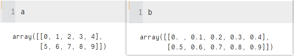
a = np.arange(10).reshape(2,5)
b = np.linspace(0,1,endpoint=False,num=10).reshape(2,5)
(1) Using vstack function to realize array vertical combination: np.vstack((arr1,arr2))
np.vstack((a,b))#Merge vertically, stack up and down
array([[0. , 1. , 2. , 3. , 4. ],
       [5. , 6. , 7. , 8. , 9. ],
       [0. , 0.1, 0.2, 0.3, 0.4],
       [0.5, 0.6, 0.7, 0.8, 0.9]])
(2) Using hstack function to realize array horizontal combination: np.hstack((arr1,arr2))
np.hstack((a,b))#Horizontal merge, left and right splicing
array([[0. , 1. , 2. , 3. , 4. , 0. , 0.1, 0.2, 0.3, 0.4],
       [5. , 6. , 7. , 8. , 9. , 0.5, 0.6, 0.7, 0.8, 0.9]])
(3) Using concatenate function to realize array vertical combination
np.concatenate((a,b),axis=0)#Equivalent to vstack(), default axis=0
array([[0. , 1. , 2. , 3. , 4. ],
       [5. , 6. , 7. , 8. , 9. ],
       [0. , 0.1, 0.2, 0.3, 0.4],
       [0.5, 0.6, 0.7, 0.8, 0.9]])
(4) Using concatenate function to realize array horizontal combination
np.concatenate((a,b),axis=1)#Equivalent to hstack()
array([[0. , 1. , 2. , 3. , 4. , 0. , 0.1, 0.2, 0.3, 0.4],
       [5. , 6. , 7. , 8. , 9. , 0.5, 0.6, 0.7, 0.8, 0.9]])
4.5 cutting array
arr = np.arange(12).reshape(3,4)
arr
array([[ 0,  1,  2,  3],
       [ 4,  5,  6,  7],
       [ 8,  9, 10, 11]])
(1) The hsplit function and split function are used to realize horizontal array segmentation
np.hsplit(arr, 4)
[array([[0],
        [4],
        [8]]), array([[1],
        [5],
        [9]]), array([[ 2],
        [ 6],
        [10]]), array([[ 3],
        [ 7],
        [11]])]
Equivalent to:
np.split(arr,4,axis=1)
[array([[0],
        [4],
        [8]]), array([[1],
        [5],
        [9]]), array([[ 2],
        [ 6],
        [10]]), array([[ 3],
        [ 7],
        [11]])]
(2) Use vsplit function and split function to achieve vertical array segmentation:
np.vsplit(arr,3)
[array([[0, 1, 2, 3]]), array([[4, 5, 6, 7]]), array([[ 8, 9, 10, 11]])]
Equivalent to:
np.split(arr,3,axis=0)
[array([[0, 1, 2, 3]]), array([[4, 5, 6, 7]]), array([[ 8, 9, 10, 11]])]

