abstract
The first part of this section mainly reviews the computational logic of RNN model, the difference between RNN model and MLP, as well as the characteristics, defects and solutions of RNN (gradient clipping), and then takes the text data set as the training sample to realize the RNN prediction model from scratch, and the concise implementation with the help of deep learning framework. The second is to learn the gating loop unit (GRU), construct the structure of reset gate and update gate, and calculate the candidate hidden state and hidden state. GRU model can better capture the long-term dependencies in the sequence, and it is simpler than LSTM. And continue to use the text data set as the sample code to realize the prediction of GRU model. The third is the code implementation of LSTM model. Continue to use text data set and deep learning framework to complete training and prediction concisely and clearly.
1. RNN cyclic neural network
First, hidden layer and hidden state refer to two distinct concepts. Hidden layer is a hidden layer understood from the perspective of observation on the path from input to output, and hidden state is the input defined from the technical perspective of anything done in a given step, and these states can only be calculated from the data of previous time steps.
Recurrent neural networks (RNNs) are neural networks with hidden states.
1.1 neural network without hidden state
First look at the multi-layer perceptron (MLP/ANN) with only a single hidden layer. Set the activation function of the hidden layer as ϕ \phi ϕ. Given a small batch of samples X ∈ R n × d \mathbf{X} \in \mathbb{R}^{n \times d} X∈Rn × d. The batch size is n n n. The input dimension is d d d. Then hide the output of the layer H ∈ R n × h \mathbf{H} \in \mathbb{R}^{n \times h} h∈Rn × h is calculated by the following formula:
H = ϕ ( X W x h + b h ) . \mathbf{H} = \phi(\mathbf{X} \mathbf{W}_{xh} + \mathbf{b}_h). H=ϕ(XWxh+bh).
The hidden layer weight parameter is W x h ∈ R d × h \mathbf{W}_{xh} \in \mathbb{R}^{d \times h} Wxh∈Rd × h. The offset parameter is b h ∈ R 1 × h \mathbf{b}_h \in \mathbb{R}^{1 \times h} bh∈R1 × h. And the number of hidden units is h h h.
Use the hidden variable 𝐇 as input to the output layer. The output layer is given by the following formula:
O = H W h q + b q , \mathbf{O} = \mathbf{H} \mathbf{W}_{hq} + \mathbf{b}_q, O=HWhq+bq,
Among them, O ∈ R n × q \mathbf{O} \in \mathbb{R}^{n \times q} O∈Rn × q is the output variable, W h q ∈ R h × q \mathbf{W}_{hq} \in \mathbb{R}^{h \times q} Whq∈Rh × q is the weight parameter, b q ∈ R 1 × q \mathbf{b}_q \in \mathbb{R}^{1 \times q} bq∈R1 × q is the offset parameter of the output layer. If it's a classification problem, we can use softmax ( O ) \text{softmax}(\mathbf{O}) softmax(O) to calculate the probability distribution of the output category.
1.2 recurrent neural network with hidden state
about
n
n
A small batch of n sequence samples,
X
t
\mathbf{X}_t
Each row of Xt , corresponds to a time step from the sequence
t
t
One sample at t. Next, use
H
t
∈
R
n
×
h
\mathbf{H}_t \in \mathbb{R}^{n \times h}
Ht∈Rn × h represents time step
t
t
Hidden variables of t. Different from the multi-layer perceptron, we save the hidden variables of the previous time step here
H
t
−
1
\mathbf{H}_{t-1}
Ht − 1, and a new weight parameter is introduced
W
h
h
∈
R
h
×
h
\mathbf{W}_{hh} \in \mathbb{R}^{h \times h}
Whh∈Rh × h to describe how to use the hidden variables of the previous time step in the current time step. Specifically, the calculation of the hidden variable of the current time step is determined by the input of the current time step together with the hidden variable of the previous time step:
H
t
=
ϕ
(
X
t
W
x
h
+
H
t
−
1
W
h
h
+
b
h
)
.
\mathbf{H}_t = \phi(\mathbf{X}_t \mathbf{W}_{xh} + \mathbf{H}_{t-1} \mathbf{W}_{hh} + \mathbf{b}_h).
Ht=ϕ(XtWxh+Ht−1Whh+bh).
Hidden variables from adjacent time steps H t \mathbf{H}_t Ht ^ and H t − 1 \mathbf{H}_{t-1} According to the relationship between Ht − 1, these variables capture and retain the historical information of the sequence until its current time step, such as the state or memory of the neural network under the current time step. Therefore, such hidden variables are called hidden state.
The output of the output layer is similar to the calculation in the multi-layer perceptron:
O t = H t W h q + b q . \mathbf{O}_t = \mathbf{H}_t \mathbf{W}_{hq} + \mathbf{b}_q. Ot=HtWhq+bq.
Weight of output layer W h q ∈ R h × q \mathbf{W}_{hq} \in \mathbb{R}^{h \times q} Whq∈Rh × q and offset b q ∈ R 1 × q \mathbf{b}_q \in \mathbb{R}^{1 \times q} bq∈R1×q.
Note: the recurrent neural network always uses these model parameters even at different time steps. Therefore, the parameter overhead of recurrent neural network will not increase with the increase of time step.
The computational logic of the recurrent neural network is briefly described below:
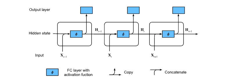
The calculation of hidden status can be regarded as:
1. Splice current time step
t
t
t Input
X
t
\mathbf{X}_t
Xt # and previous time step
t
−
1
t-1
Hidden state of t − 1
H
t
−
1
\mathbf{H}_{t-1}
Ht−1;
2. The result of splicing is fed into the function with activation
ϕ
\phi
ϕ Full connection layer. The output of the full connection layer is the current time step
t
t
Hidden state of t
H
t
\mathbf{H}_t
Ht.
3. Current time step
t
t
Hidden state of t
H
t
\mathbf{H}_t
Ht # will participate in the calculation of the next time step
t
+
1
t+1
Hidden state of t+1
H
t
+
1
\mathbf{H}_{t+1}
Ht+1. and
H
t
\mathbf{H}_t
Ht # will also be sent to the fully connected output layer for calculating the current time step
t
t
Output of t
O
t
\mathbf{O}_t
Ot.
Then use a simple code fragment to implement:
Hidden state
X
t
W
x
h
+
H
t
−
1
W
h
h
\mathbf{X}_t \mathbf{W}_{xh} + \mathbf{H}_{t-1} \mathbf{W}_{hh}
The calculation of Xt Wxh + Ht − 1 Whh is equivalent to
X
t
\mathbf{X}_t
Xt , and
H
t
−
1
\mathbf{H}_{t-1}
Splicing and of Ht − 1
W
x
h
\mathbf{W}_{xh}
Wxh} and
W
h
h
\mathbf{W}_{hh}
Matrix multiplication of wh.
import torch
from d2l import torch as d2l

X, W_xh = torch.normal(0, 1, (3, 1)), torch.normal(0, 1, (1, 4))
H, W_hh = torch.normal(0, 1, (3, 4)), torch.normal(0, 1, (4, 4))
torch.matmul(X, W_xh) + torch.matmul(H, W_hh)

###1. Calculate the output matrix according to the formula
tensor([[ 0.6291, -4.1447, -0.5398,  2.7443],
        [-0.0836, -0.7853,  0.1801, -0.9263],
        [-2.8293,  4.8625,  2.6801,  1.1304]])

### 2. Multiply and output the same matrix after matrix splicing
torch.matmul(torch.cat((X, H), 1), torch.cat((W_xh, W_hh), 0))

tensor([[ 0.6291, -4.1447, -0.5398,  2.7443],
        [-0.0836, -0.7853,  0.1801, -0.9263],
        [-2.8293,  4.8625,  2.6801,  1.1304]])
1.3 take text dataset as an example to realize RNN prediction model
Don't look closely, this is realized from scratch! There are no functions provided by the advanced API of the deep learning framework.
1.3.1 reading data
Taking the time machine data set as the training data, the model will be trained on the time machine data set. We first read the data set:
%matplotlib inline
import math
import torch
from torch import nn
from torch.nn import functional as F
from d2l import torch as d2l

batch_size, num_steps = 32, 35
# Parameter batch_size specifies the number of neutron sequence samples in each small batch, and the parameter num_steps is the number of predefined time steps in each subsequence.
# Read the time machine data set and reference the total function load defined before_ data_ time_ machine(),batch_ Size = batch size, num_steps = time step
train_iter, vocab = d2l.load_data_time_machine(batch_size, num_steps)
1.3.2 single heat code (word)
Turn a subscript into a vector for neural network processing. That is, one hot:
F.one_hot(torch.tensor([0, 2]), len(vocab))   # Total vocab parts of speech length = 28
## output
tensor([[1, 0, 0, 0, 0, 0, 0, 0, 0, 0, 0, 0, 0, 0, 0, 0, 0, 0, 0, 0, 0, 0, 0, 0,
         0, 0, 0, 0],
        [0, 0, 1, 0, 0, 0, 0, 0, 0, 0, 0, 0, 0, 0, 0, 0, 0, 0, 0, 0, 0, 0, 0, 0,
         0, 0, 0, 0]])
Convert the input dimension to obtain the output with the shape (time steps, batch size, vocabulary size). This will make it easier for us to update the hidden state of small batch data step by step through the outermost dimension.
X = torch.arange(10).reshape((2, 5))
F.one_hot(X.T, 28).shape # After transposing, you can iterate in time steps

##Shape of output batch data
torch.Size([5, 2, 28])
1.3.3 initialize model parameters of RNN
Number of hidden cells num_hiddens is an adjustable hyperparameter. When training the language model, the input and output come from the same vocabulary. Therefore, they have the same dimension, that is, the size of the vocabulary.
 # 1. Define get of learnable parameters_ Params function
def get_params(vocab_size, num_hiddens, device):
    num_inputs = num_outputs = vocab_size #Both input and output are equal to the vocabulary size

    def normal(shape): # Define normal function, initialization function with mean value of 0 and variance of 1 * 0.01
        return torch.randn(size=shape, device=device) * 0.01

    # Hidden layer parameters
    W_xh = normal((num_inputs, num_hiddens))
    W_hh = normal((num_hiddens, num_hiddens))
    b_h = torch.zeros(num_hiddens, device=device)

    # Output layer parameters
    W_hq = normal((num_hiddens, num_outputs))
    b_q = torch.zeros(num_outputs, device=device)

    # Additional gradient
    params = [W_xh, W_hh, b_h, W_hq, b_q]
    for param in params:
        param.requires_grad_(True)
    return params
1.3.4 define RNN model
Define an init_ rnn_ The state function returns a hidden state during initialization, and a hidden variable is also required at time 0.
# 2. Initialize hidden state
def init_rnn_state(batch_size, num_hiddens, device):  # At time 0, initialize the hidden state, 0 / random.
return (torch.zeros((batch_size, num_hiddens), device=device), )
The next step is the calculation. The following rnn function defines how to calculate the hidden state and output in a time step
# The rnn function defines how to calculate the hidden state and output in a time step
def rnn(inputs, state, params):
    # input is a three-dimensional tensor (time step, batch size, vocabulary size)
    W_xh, W_hh, b_h, W_hq, b_q = params
    H, = state
    outputs = []
    for X in inputs:   # `Shape of X: (` batch size ',' thesaurus size '),
        # That is, traverse one by one (from T1, T2,... T10) along the dimension of the time step
        H = torch.tanh(torch.mm(X, W_xh)
                       + torch.mm(H, W_hh)
                       + b_h)   # tanh function as activation function
        Y = torch.mm(H, W_hq) + b_q
        outputs.append(Y)
    return torch.cat(outputs, dim=0), (H,)
# torch.cat() is to splice the output of each time step. n matrices are spliced according to dim = 0 (vertically), and the hidden state is updated (why do you splice like this?)
Special attention: the cyclic neural network model realizes the cycle through the outermost dimension (time step) of inputs, so as to update the hidden state H of small batch data step by step.
1.3.5 create a class to wrap these functions
class RNNModelScratch: #@save
    """Cyclic neural network model implemented from scratch"""
    def __init__(self, vocab_size, num_hiddens, device,
                 get_params, init_state, forward_fn):
        self.vocab_size, self.num_hiddens = vocab_size, num_hiddens
        self.params = get_params(vocab_size, num_hiddens, device)
        self.init_state, self.forward_fn = init_state, forward_fn

    def __call__(self, X, state):  # X-quantization
        X = F.one_hot(X.T, self.vocab_size).type(torch.float32)
        return self.forward_fn(X, state, self.params)   ## Forward here_ FN (,,) actually defines the rnn function above

    def begin_state(self, batch_size, device):
        return self.init_state(batch_size, self.num_hiddens, device) # Call init_state function
Check whether the output has the correct shape, for example, whether the dimension of the hidden state remains unchanged.
num_hiddens = 512 # Hidden layer size
net = RNNModelScratch(len(vocab), num_hiddens, d2l.try_gpu(), get_params, # Learnable parameters
init_rnn_state, rnn) # Model type

state = net.begin_state(X.shape[0], d2l.try_gpu()) # Initialize hidden state
Y, new_state = net(X.to(d2l.try_gpu()), state)
Y.shape, len(new_state), new_state[0].shape
# Output shape, and shape in hidden state
(torch.Size([10, 28]), 1, torch.Size([2, 512]))
The output shape is (time steps) × Batch size (vocabulary size) output Y is spliced (the one that is spliced vertically), while the shape of the hidden state remains unchanged, that is (batch size, number of hidden units).
1.3.6 gradient cutting
Gradient clipping is applied to solve the problem of gradient explosion caused by optimization. The gradient 𝐠 is clipped by projecting the gradient 𝐠 back to the ball with a given radius (e.g. 𝜃). The following formula:

The gradient norm will never exceed 𝜃, and the updated gradient is completely aligned with the original direction of 𝐠. It also has a side effect worth having, that is, limiting the influence of any given small batch data (and any given sample) on the parameter vector, which gives the model a certain degree of stability. Gradient clipping provides a fast method to repair gradient explosion.
# Define a function to crop the gradient of the model
def grad_clipping(net, theta):  #@save
    """Crop gradient."""
    if isinstance(net, nn.Module):
        params = [p for p in net.parameters() if p.requires_grad]
    else:
        params = net.params  # Take all parameters of the network layer that can participate in training
    norm = torch.sqrt(sum(torch.sum((p.grad ** 2)) for p in params))  # The parameter p of all layers, sum and open root sign, is to find L2 norm
    if norm > theta: # Prevent excessive gradient
        for param in params:
            param.grad[:] *= theta / norm
1.3.7 prediction (prediction before training)
Define a prediction function to generate new characters after prefix
def predict_ch8(prefix, num_preds, net, vocab, device):  #@save  ,num_preds predicts several characters (words), net is a trained model, and vocab can map into real string values.
    """stay`prefix`Generate new characters after."""
    state = net.begin_state(batch_size=1, device=device)
    outputs = [vocab[prefix[0]]]   ## Put the first word or character into vocab, get the corresponding integer subscript, and put it into output
    get_input = lambda: torch.tensor([outputs[-1]], device=device).reshape((1, 1))
    for y in prefix[1:]:  # Preheating period
        _, state = net(get_input(), state)
        outputs.append(vocab[y])
    for _ in range(num_preds):   # Forecast ` num_preds ` step
        y, state = net(get_input(), state)  # Take the last of the last output as the next input, and y is the vector of 1*vocab.size
        outputs.append(int(y.argmax(dim=1).reshape(1))) #Take out the maximum coordinate of y, replace it with a scalar, and take it to outputs
    return ''.join([vocab.idx_to_token[i] for i in outputs])
1.3.8 start training
- Define a function to train the model in an iteration cycle
#@save
def train_epoch_ch8(net, train_iter, loss, updater, device, use_random_iter): # All parameters are available
    """The training model has one iteration cycle"""
    state, timer = None, d2l.Timer()
    metric = d2l.Accumulator(2)  # Sum of training losses, number of morphemes
    for X, Y in train_iter:
        if state is None or use_random_iter:
            # Initialize at first iteration or when using random sampling ` state`
            state = net.begin_state(batch_size=X.shape[0], device=device)
        else:
            if isinstance(net, nn.Module) and not isinstance(state, tuple):
                # `state ` is a tensor for ` nn.GRU '
                state.detach_()
            else:
                # `state ` is a tensor for ` nn.LSTM 'or for our model implemented from scratch
                for s in state:
                    s.detach_()
        y = Y.T.reshape(-1) # Transpose Y and pull it into a vector
        X, y = X.to(device), y.to(device)
        y_hat, state = net(X, state)
        l = loss(y_hat, y.long()).mean()  # This explains why y splicing is essentially a multi classification problem in the view of loss function
        if isinstance(updater, torch.optim.Optimizer):
            updater.zero_grad()
            l.backward()
            grad_clipping(net, 1)
            updater.step()
        else:
            l.backward()
            grad_clipping(net, 1)
            # Because the 'mean' function has been called
            updater(batch_size=1)
        metric.add(l * y.numel(), y.numel())
    return math.exp(metric[0] / metric[1]), metric[1] / timer.stop() # The average cross entropy and confusion degree are obtained
- Training function of recurrent neural network model
#@save
def train_ch8(net, train_iter, vocab, lr, num_epochs, device,
              use_random_iter=False):
    """Training model"""
    loss = nn.CrossEntropyLoss()
    animator = d2l.Animator(xlabel='epoch', ylabel='perplexity',
                            legend=['train'], xlim=[10, num_epochs])
    # initialization
    if isinstance(net, nn.Module):
        updater = torch.optim.SGD(net.parameters(), lr)
    else:
        updater = lambda batch_size: d2l.sgd(net.params, lr, batch_size)
    predict = lambda prefix: predict_ch8(prefix, 50, net, vocab, device)
    # Training and forecasting
    for epoch in range(num_epochs):
        ppl, speed = train_epoch_ch8(
            net, train_iter, loss, updater, device, use_random_iter)
        if (epoch + 1) % 10 == 0:
            print(predict('time traveller'))
            animator.add(epoch + 1, [ppl])
    print(f'Confusion degree {ppl:.1f}, {speed:.1f} Lexical element/second {str(device)}')
    print(predict('time traveller'))
    print(predict('traveller'))
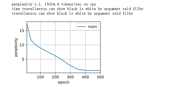
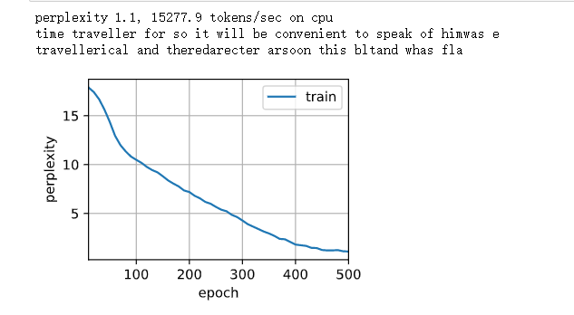
Sequential partition sampling is adopted to train, and the prediction results are as follows:
num_epochs, lr = 500, 1
train_ch8(net, train_iter, vocab, lr, num_epochs, d2l.try_gpu())
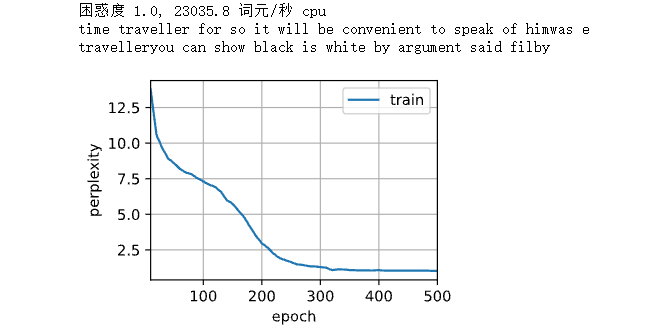
It can be seen that the degree of confusion is very good. For this RNN model, it is predicted by characters. The overall prediction effect seems good, but there are still many problems, such as unclear semantics, etc.
Then, the random sampling method is used for training:
The prediction results are as follows
train_ch8(net, train_iter, vocab, lr, num_epochs, d2l.try_gpu(),
          use_random_iter=True)
It can be seen that the confusion increases and the calculation becomes complex, because the hidden state needs to be recalculated every time. The prediction results are similar to the above, and the performance is fairly good.
The time machine data set is too small. In the future, you can increase the training sample set to see if the results can be improved.
1.4 concise implementation of RNN text prediction model
This section will show how to use the functions provided by the advanced API of the deep learning framework to more effectively implement the same language model. Still start by reading the time machine dataset.
import torch
from torch import nn
from torch.nn import functional as F
from d2l import torch as d2l

batch_size, num_steps = 32, 35  #Batch size, time step
train_iter, vocab = d2l.load_data_time_machine(batch_size, num_steps)
Define model
- A single hidden layer recurrent neural network layer RNN with 256 hidden units is constructed_ layer:
num_hiddens = 256
rnn_layer = nn.RNN(len(vocab), num_hiddens)
- The tensor is used to initialize the hidden state. Its shape is (number of hidden layers, batch size, number of hidden units)
state = torch.zeros((1, batch_size, num_hiddens)) #Initialize hidden state
state.shape

#output
torch.Size([1, 32, 256])
- Through a hidden state and an input, we can calculate the output with the updated hidden state.
X = torch.rand(size=(num_steps, batch_size, len(vocab)))
Y, state_new = rnn_layer(X, state)
# Y is actually the y of the hidden layer, not the y of the output layer
#rnn_layer's "output" (Y) does not involve the calculation of the output layer: it refers to the hidden states of each time step, which can be used as the input of subsequent output layers.
Y.shape, state_new.shape
# output
(torch.Size([35, 32, 256]), torch.Size([1, 32, 256]))
-
An RNNModel class is defined for a complete cyclic neural network model
rnn_layer contains only hidden loop layers, and we also need to create a separate output layer.
class RNNModel(nn.Module):
    """Cyclic neural network model."""
    def __init__(self, rnn_layer, vocab_size, **kwargs):
        super(RNNModel, self).__init__(**kwargs) # super().__init__ () derived method.
        self.rnn = rnn_layer
        self.vocab_size = vocab_size
        self.num_hiddens = self.rnn.hidden_size
        # If RNN is bidirectional, ` num_directions ` should be 2, otherwise it should be 1.
        if not self.rnn.bidirectional:
            self.num_directions = 1#Unidirectional RNN model
            self.linear = nn.Linear(self.num_hiddens, self.vocab_size)# Construct linear output layer
        else:
            self.num_directions = 2 # Bidirectional RNN model
            self.linear = nn.Linear(self.num_hiddens * 2, self.vocab_size)

    def forward(self, inputs, state):
        X = F.one_hot(inputs.T.long(), self.vocab_size)
        X = X.to(torch.float32) #
        Y, state = self.rnn(X, state)
        # Y is the shape of the middle hidden layer (time step, batch size, number of hidden cells)

        # The full connection layer first changes the shape of 'Y' to (` time steps ` * ` batch size `, ` number of hidden units')

        output = self.linear(Y.reshape((-1, Y.shape[-1])))
         # Its output shape is (` time steps ` * ` batch size `, ` thesaurus size `)
        return output, state

    def begin_state(self, device, batch_size=1):
        if not isinstance(self.rnn, nn.LSTM):
            # `nn.GRU ` Take tensor as hidden state
            return  torch.zeros((self.num_directions * self.rnn.num_layers,
                                 batch_size, self.num_hiddens),
                                device=device)
        else:
            # `nn.LSTM ` Take tensor as hidden state
            return (
                torch.zeros((
                self.num_directions * self.rnn.num_layers,
                batch_size, self.num_hiddens), device=device),
                    torch.zeros((
                        self.num_directions * self.rnn.num_layers,
                        batch_size, self.num_hiddens), device=device)
            )
- Training and prediction
Prediction based on a model with random weight:
device = d2l.try_gpu()
net = RNNModel(rnn_layer, vocab_size=len(vocab))
net = net.to(device)
d2l.predict_ch8('time traveller', 10, net, vocab, device)
##Forecast results (random)
'time travellerzzzzzzzzzz'
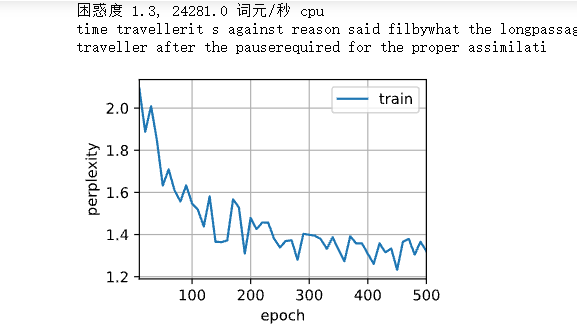
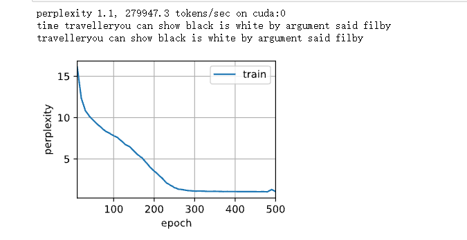
Call train with the super parameters defined in the previous section (implemented from zero)_ Ch8, and use the advanced API to train the model.
num_epochs, lr = 500, 1
d2l.train_ch8(net, train_iter, vocab, lr, num_epochs, device)
The predicted results are as follows:
It can be seen that the model using the deep learning framework can optimize the code, so the time to reduce the degree of confusion is shortened.
Note: using the framework (without avoiding the initialization state) only avoids the initialization weight. How to calculate the RNN is different from rnn_layer has no output layer, and the output y is not the predicted result y.
2. Door control circulation unit (GRU)
The main difference between GRU and ordinary RNN is that GRU has hidden gating and soft control. There are special mechanisms to determine when the hidden state should be updated and when the hidden state should be reset. These mechanisms are learnable.
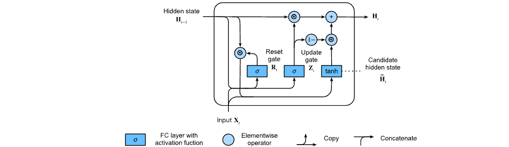
2.1 reset door and update door
The structure of reset gate and update gate is shown in the following figure:
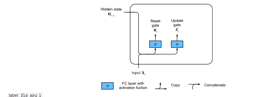
The input is given by the input of the current time step and the hidden state of the previous time step, and the output of the two gates is given by the two fully connected layers using the sigmoid activation function.
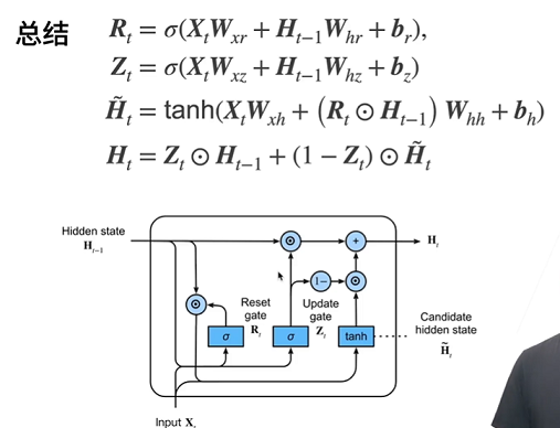
Suppose the input is a small batch X t ∈ R n × d \mathbf{X}_t \in \mathbb{R}^{n \times d} Xt∈Rn × d (number of samples: n n n. Enter number: d d d) , the hidden state of the previous time step is H t − 1 ∈ R n × h \mathbf{H}_{t-1} \in \mathbb{R}^{n \times h} Ht−1∈Rn × h (number of hidden units: h h h). Then reset the door R t ∈ R n × h \mathbf{R}_t \in \mathbb{R}^{n \times h} Rt∈Rn × h and update doors Z t ∈ R n × h \mathbf{Z}_t \in \mathbb{R}^{n \times h} Zt∈Rn × h is calculated as follows:
R t = σ ( X t W x r + H t − 1 W h r + b r ) , Z t = σ ( X t W x z + H t − 1 W h z + b z ) , \begin{aligned} \mathbf{R}_t = \sigma(\mathbf{X}_t \mathbf{W}_{xr} + \mathbf{H}_{t-1} \mathbf{W}_{hr} + \mathbf{b}_r),\\ \mathbf{Z}_t = \sigma(\mathbf{X}_t \mathbf{W}_{xz} + \mathbf{H}_{t-1} \mathbf{W}_{hz} + \mathbf{b}_z), \end{aligned} Rt=σ(XtWxr+Ht−1Whr+br),Zt=σ(XtWxz+Ht−1Whz+bz),
among W x r , W x z ∈ R d × h \mathbf{W}_{xr}, \mathbf{W}_{xz} \in \mathbb{R}^{d \times h} Wxr,Wxz∈Rd × h and W h r , W h z ∈ R h × h \mathbf{W}_{hr}, \mathbf{W}_{hz} \in \mathbb{R}^{h \times h} Whr,Whz∈Rh × h is the weight parameter, b r , b z ∈ R 1 × h \mathbf{b}_r, \mathbf{b}_z \in \mathbb{R}^{1 \times h} br,bz∈R1 × h is the offset parameter.
Note: the broadcast mechanism will be triggered during the summation process, and the sigmoid function will be used to convert the input value to the interval ( 0 , 1 ) (0, 1) (0,1).
2.2 candidate hidden status
The door will be reset R t \mathbf{R}_t Rt ^ is integrated with the conventional implicit state update mechanism of RNN t t Candidate hidden state of t H ~ t ∈ R n × h \tilde{\mathbf{H}}_t \in \mathbb{R}^{n \times h} H~t∈Rn×h.
H ~ t = tanh ( X t W x h + ( R t ⊙ H t − 1 ) W h h + b h ) , \tilde{\mathbf{H}}_t = \tanh(\mathbf{X}_t \mathbf{W}_{xh} + \left(\mathbf{R}_t \odot \mathbf{H}_{t-1}\right) \mathbf{W}_{hh} + \mathbf{b}_h), H~t=tanh(XtWxh+(Rt⊙Ht−1)Whh+bh),
among W x h ∈ R d × h \mathbf{W}_{xh} \in \mathbb{R}^{d \times h} Wxh∈Rd × h and W h h ∈ R h × h \mathbf{W}_{hh} \in \mathbb{R}^{h \times h} Whh∈Rh × h is the weight parameter, b h ∈ R 1 × h \mathbf{b}_h \in \mathbb{R}^{1 \times h} bh∈R1 × h is the offset term.
Note: Symbols ⊙ \odot ⊙ is the hada code product (by element product) operator. The tanh nonlinear activation function is used to ensure that the values in the candidate hidden state remain in the interval ( − 1 , 1 ) (-1, 1) (− 1,1).
2.3 hidden status
Combined renewal door Z t \mathbf{Z}_t The effect of Zt. This determines the new hidden state H t ∈ R n × h \mathbf{H}_t \in \mathbb{R}^{n \times h} Ht∈Rn × To what extent is h the old state H t − 1 \mathbf{H}_{t-1} Ht − 1, and new candidate status H ~ t \tilde{\mathbf{H}}_t Usage of H~t ^. Update door Z t \mathbf{Z}_t Zt , only required in H t − 1 \mathbf{H}_{t-1} Ht − 1 and H ~ t \tilde{\mathbf{H}}_t This goal can be achieved by the convex combination of elements between H~t ^. This leads to the final update formula of the gating cycle unit:
H t = Z t ⊙ H t − 1 + ( 1 − Z t ) ⊙ H ~ t . \mathbf{H}_t = \mathbf{Z}_t \odot \mathbf{H}_{t-1} + (1 - \mathbf{Z}_t) \odot \tilde{\mathbf{H}}_t. Ht=Zt⊙Ht−1+(1−Zt)⊙H~t.
Reset the door and update the calculation flow after the door works as follows:

The gated circulation unit has the following two remarkable characteristics:
- Resetting the gate helps capture short-term dependencies in the sequence
- Update gates help capture long-term dependencies in sequences
2.4 code implementation GRU model
2.4.1 start from scratch
- Read the code of the data set (take the text as the training sample)
import torch
from torch import nn
from d2l import torch as d2l

batch_size, num_steps = 32, 35
train_iter, vocab = d2l.load_data_time_machine(batch_size, num_steps)
- Initialize model parameters
The weight is extracted from the Gaussian distribution with standard deviation of 0.01, the offset term is set to 0, and the super parameter num_hiddens defines the number of hidden units and instantiates all weights and offsets related to update gate, reset gate, candidate hidden state and output layer.
(the same as the previous RNN initialization parameters, but the parameters are increased)
def get_params(vocab_size, num_hiddens, device):
    num_inputs = num_outputs = vocab_size

    def normal(shape):
        return torch.randn(size=shape, device=device)*0.01

    def three():
        return (normal((num_inputs, num_hiddens)),
                normal((num_hiddens, num_hiddens)),
                torch.zeros(num_hiddens, device=device))

    W_xz, W_hz, b_z = three()  # Update door parameters
    W_xr, W_hr, b_r = three()  # Reset door parameters
    # GRU has more parameters in the above two lines than RNN

    W_xh, W_hh, b_h = three()  # Candidate hidden state parameters
    # Output layer parameters
    W_hq = normal((num_hiddens, num_outputs))
    b_q = torch.zeros(num_outputs, device=device)
    # Additional gradient
    params = [W_xz, W_hz, b_z, W_xr, W_hr, b_r, W_xh, W_hh, b_h, W_hq, b_q]
    for param in params:
        param.requires_grad_(True)
    return params
- Defines the initialization function of the hidden state
def init_gru_state(batch_size, num_hiddens, device):
    return (torch.zeros((batch_size, num_hiddens), device=device), )
- Define gating cycle unit model
The structure of the model is the same as the basic cyclic neural network unit, but the weight update formula is more complex.
def gru(inputs, state, params):
    W_xz, W_hz, b_z, W_xr, W_hr, b_r, W_xh, W_hh, b_h, W_hq, b_q = params # A hidden layer has 11 parameters
    H, = state
    outputs = []
    for X in inputs:  # Take out X every time

        Z = torch.sigmoid((X @ W_xz) + (H @ W_hz) + b_z)
        R = torch.sigmoid((X @ W_xr) + (H @ W_hr) + b_r)
        H_tilda = torch.tanh((X @ W_xh) + ((R * H) @ W_hh) + b_h)
        H = Z * H + (1 - Z) * H_tilda
        Y = H @ W_hq + b_q

        outputs.append(Y)
    return torch.cat(outputs, dim=0), (H,)
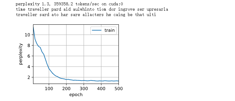
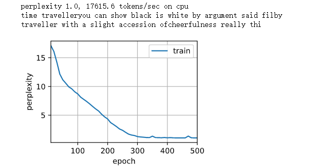
- Training and prediction
vocab_size, num_hiddens, device = len(vocab), 256, d2l.try_gpu()
num_epochs, lr = 500, 1
model = d2l.RNNModelScratch(len(vocab), num_hiddens, device, get_params,
 init_gru_state, gru) # Call the previously defined RNNModelScratch() function
d2l.train_ch8(model, train_iter, vocab, lr, num_epochs, device)#Call the previous training function train_ch8()
The predicted results are as follows:
2.4.2 concise implementation
Using the framework of deep learning, the gated loop unit model can be instantiated directly, and the code runs faster.
num_inputs = vocab_size
gru_layer = nn.GRU(num_inputs, num_hiddens)
model = d2l.RNNModel(gru_layer, len(vocab))
model = model.to(device)
d2l.train_ch8(model, train_iter, vocab, lr, num_epochs, device)
result:
3. Comparison between LSTM model review and GRU
LSTM calculation logic flow chart:
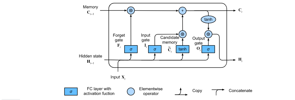
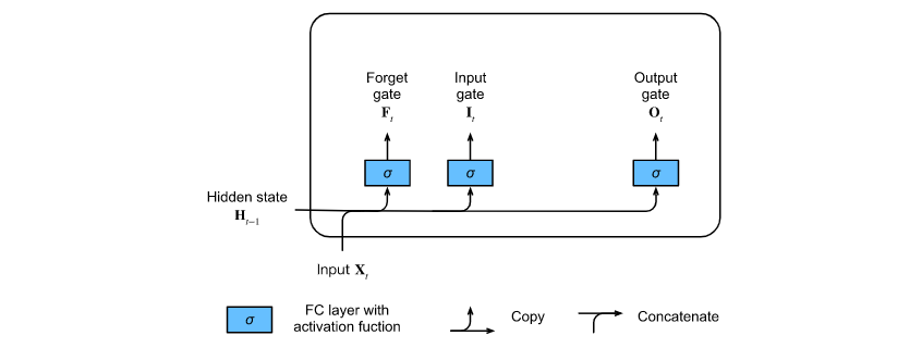
3.1 input gate, forgetting gate and output gate
The input of the current time step and the hidden state of the previous time step are sent into the long-term and short-term memory network gate as data. They are processed by three full connection layers with sigmoid activation function to calculate the values of input gate, forgetting gate and output gate. Therefore, the values of these three gates are in the range of (0,1). As shown in the figure:
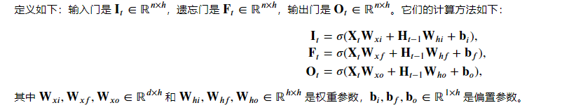
3.2 candidate memory units
The candidate memory unit C uses the tanh function as the activation function, and the value range of the function is (− 1,1). The calculation is similar to the hidden state Ht in RNN, but there will be two states in LSTM.

3.3 memory unit
In GRU, there is a mechanism to control input and forgetting (or skipping). Similarly, in LSTM, there are two doors for such purposes:
1. The input gate controls how many candidate hidden states are used
C
~
t
\tilde{\mathbf{C}}_t
New data of C~t;
2. The forgetting gate controls how many old memory units are retained × The content of.
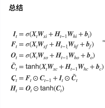
Using the same technique of multiplying by elements as before, the following update formula is obtained:

3.4 hidden status
Where the output gate works to ensure that the value of 𝐇 𝑡 is always within the interval (− 1,1), the tanh function needs to be added as the activation function.
In short, this mechanism is to either focus on the current Xt, pay more attention to the previous things, or reset the current information.
Output:
Y
t
=
H
t
W
(
h
q
)
+
b
q
Y_t=H_t W_(hq)+b_q
Yt=HtW(hq)+bq
Comparison - GRU calculation logic flow:
4. Code implementation LSTM
4.1 reading data sets
import torch
from torch import nn
from d2l import torch as d2l

batch_size, num_steps = 32, 35
train_iter, vocab = d2l.load_data_time_machine(batch_size, num_steps)
4.2 initialization model parameters
def get_lstm_params(vocab_size, num_hiddens, device):
    num_inputs = num_outputs = vocab_size

    def normal(shape):  # Customize an initialization function normal()
        return torch.randn(size=shape, device=device)*0.01

    def three():
        return (normal((num_inputs, num_hiddens)),
                normal((num_hiddens, num_hiddens)),
                torch.zeros(num_hiddens, device=device))

    W_xi, W_hi, b_i = three()  # Enter door parameters
    W_xf, W_hf, b_f = three()  # Forgetting gate parameters
    W_xo, W_ho, b_o = three()  # Output gate parameters
    W_xc, W_hc, b_c = three()  # Candidate memory cell parameters

    # Output layer parameters
    W_hq = normal((num_hiddens, num_outputs))
    b_q = torch.zeros(num_outputs, device=device)
    # Additional gradient
    params = [W_xi, W_hi, b_i, W_xf, W_hf, b_f, W_xo, W_ho, b_o, W_xc, W_hc,
              b_c, W_hq, b_q]
    for param in params:
        param.requires_grad_(True)
    return params
4.3 definition model
- Hide state initialization:
def init_lstm_state(batch_size, num_hiddens, device):
 return (torch.zeros((batch_size, num_hiddens), device=device),# Initialization of H, shape is (batch size, number of hidden units)
  torch.zeros((batch_size, num_hiddens), device=device))# Initialization of C, the shape is (batch size, number of hidden units)
- Define lstm() function
def lstm(inputs, state, params):
    [W_xi, W_hi, b_i, W_xf, W_hf, b_f, W_xo, W_ho, b_o, W_xc, W_hc, b_c,
     W_hq, b_q] = params
    (H, C) = state
    outputs = []
    for X in inputs:  ## The key difference between RNN and Gru LSTM lies in how the Ht hidden state is updated.
        I = torch.sigmoid((X @ W_xi) + (H @ W_hi) + b_i)
        F = torch.sigmoid((X @ W_xf) + (H @ W_hf) + b_f)
        O = torch.sigmoid((X @ W_xo) + (H @ W_ho) + b_o)
        C_tilda = torch.tanh((X @ W_xc) + (H @ W_hc) + b_c)
        C = F * C + I * C_tilda   #  *Is to multiply by element points and @ matrix multiplication
        H = O * torch.tanh(C)

        ## Output Y
        Y = (H @ W_hq) + b_q

        outputs.append(Y)
    return torch.cat(outputs, dim=0), (H, C)
4.4 training and forecasting
import os
os.environ["KMP_DUPLICATE_LIB_OK"]="TRUE"

vocab_size, num_hiddens, device = len(vocab), 256, d2l.try_gpu()

num_epochs, lr = 500, 1
model = d2l.RNNModelScratch(len(vocab), num_hiddens, device, get_lstm_params,
                            init_lstm_state, lstm)    ### Introduce RNNModelScratch class
d2l.train_ch8(model, train_iter, vocab, lr, num_epochs, device)
Result output:
4.5 simple implementation using framework
num_inputs = vocab_size
lstm_layer = nn.LSTM(num_inputs, num_hiddens) ## Differences between nn.RNN(),nn.GRU(),nn.LSTM()
model = d2l.RNNModel(lstm_layer, len(vocab)) # Hidden layer lstm_layer
model = model.to(device)
d2l.train_ch8(model, train_iter, vocab, lr, num_epochs, device)
The results are predicted as follows:
Summary and Prospect
First, the difference between MLP and RNN is that the former has no hidden state and does not have the ability to capture and retain the historical information of the sequence until its current time step, that is, it cannot capture the long-term dependency of the sequence. For the code implementation of RNN model, it is necessary to read the data set and preprocess the data. Here, it is simply processed into characters (Sample English), followed by complex data. Better processing means should be provided; With the help of the deep learning framework, the concise implementation of RNN prediction model will be faster and simpler than before.
Second, the implementation of GRU structure can better capture the dependence on the sequence with long time step distance. When the reset door is opened, the gated loop unit contains the basic loop neural network; When the update door is open, the gating cycle unit can skip the subsequence.
Third, LSTM has three types of gates: input gate, forgetting gate and output gate controlling information flow. The hidden layer output of LSTM includes "hidden state" and "memory unit". Only the hidden state is passed to the output layer, and the memory unit is completely internal information. LSTM can alleviate gradient disappearance and gradient explosion.
Now the most widely used LSTM model needs to be further improved, and how different performance will be reflected on different data training sets, and how to better process the data in order to better achieve the desired results.