We know that about 70% of the earth is covered by water. If the earth is in your hands like a small ball now, you throw it into the sky. What is the probability that the point of touchdown is the water area?

This document and code are from Here.

Let's first assume that we don't know at all how much of the earth's area is covered by water, but we find that eight of the 15 tosses are water. How do we know the posterior probability distribution of this result?

Here we use the grid approximation to divide the 0-1 interval into 1000 cells Bayes formula Calculate the posterior probability distribution:

p_grid = seq(from=0, to=1, length.out=1000)
prior = rep(1, 1000)  # When there is no prior knowledge, the uniform distribution is used directly, which corresponds to the one-to-one correspondence of P ﹣ grid
prob_data = dbinom(8, size=15, prob=p_grid)
posterior = prob_data * prior
posterior = posterior / sum(posterior)

Then we take samples from the results:

set.seed(100)
samples = sample(p_grid, prob=posterior, size=1e4, replace=TRUE)
mean(samples)

The average value of sampling is about 0.53:

> mean(samples)
[1] 0.5281364

Will the results improve when we know that most of the earth is water? We modify the prior knowledge to recalculate:

p_grid = seq(from=0, to=1, length.out=1000)
prior = c(rep(0, 500), rep(1, 500))  # It is known that the proportion of water can not be less than 0.5, so directly give 0 value
prob_data = dbinom(8, size=15, prob=p_grid)
posterior = prob_data * prior
posterior = posterior / sum(posterior)

set.seed(100)
samples2 = sample(p_grid, prob=posterior, size=1e4, replace=TRUE)
mean(samples2)

Result:

> mean(samples2)
[1] 0.6054694

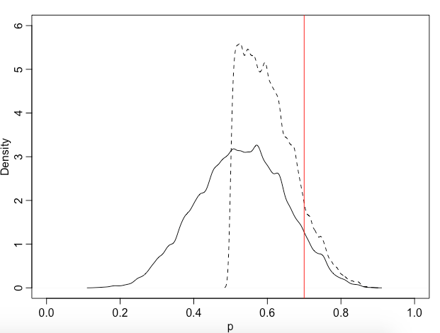
In fact, water accounts for 70%. We draw the results of the two experiments and the real values in the same picture.

library(rethinking)

dens( samples , xlab="p" , xlim=c(0,1) , ylim=c(0,6))
dens( samples2 , add=TRUE, lty=2)
abline( v=0.7 , col="red")

Now there is another problem: we want to accurately estimate the proportion of the water area of the earth, so that the interval of 99% of the posterior probability distribution of p value is within the range of 0.05, that is, the difference between the upper boundary and the lower boundary (99% interval) is 0.05, how many times do we need to throw the earth?

Next, create a function to calculate the interval difference of a posteriori distribution of p value for a given number of throws.

f = function(N) {
  p_true = 0.7
  W = rbinom(1, size = N, prob = p_true)
  p_grid = seq(from = 0, to = 1, length.out = 1000)
  prior = rep(1, 1000)
  prob_data = dbinom(W, size= N, prob = p_grid)
  posterior = prob_data * prior
  posterior = posterior / sum(posterior)
  samples = sample(p_grid, prob = posterior, size = 1e4, replace = TRUE)
  PI99 = PI(samples, 0.99)
  as.numeric(PI99[2] - PI99[1])
}

In order to make a better comparison, we set different throwing times, and we also calculate the same throwing times many times to observe the stability of the calculation results.

Nlist = c(20, 50, 100, 200, 500, 1000, 2000)
Nlist = rep(Nlist, each = 100)
width = sapply(Nlist, f)
plot(Nlist, width)
abline(h=0.05, col="red")

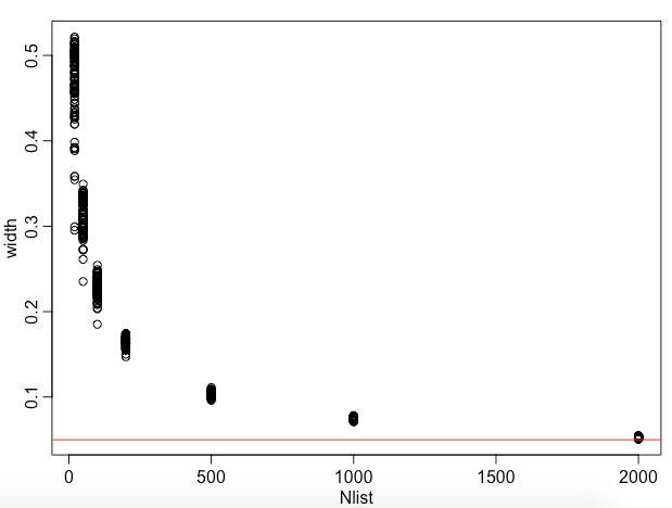
It can be seen that about 2000 times are needed, and we can stabilize the 99% interval difference at about 0.05. I guess my hands are tired, aren't they? A kind of