Author: Moxin; Date: 2019.7.25;
Learning LADRC structure:
1. Learning the relevant knowledge of PID, as the basis for learning ADRC, building modules in simulink, through adjusting parameters, to see the effect of adjusting, analyze the impact of Kp, Ki, Kd parameters on the system.
2. Introduce some knowledge of ADRC and its understanding of LADRC related parameters and their significance. Build the model with Simulink and conduct simulation test.
3. After reading the paper, we change the controlled object in Simulink and adjust the parameters to see whether the LADRC controller meets the control requirements.
4. Next, understand the basic idea of LADRC, through the programming of Matlab, to understand the realization of discrete LADRC functions, for the future application of other imitation wheat cloth as a mat. (Difficulties - take longer)
5. In future projects, LADRC will be used in practical projects. (There may be updates in the future)
Introduction to LADRC
1. Citation Papers and Their Authors'Introduction
Authors cited:
Han Jingqing: Han Jingqing, an expert in system and control, was one of the early pioneers of control theory and application in China. New guidance concepts and methods in interception problems are put forward by using optimal control theory; the development and research of computer aided design software for control systems are first promoted in China; the fertility base method for calculating population "total fertility rate" is creatively put forward; and the ADRC technology is created for the control theory and response of our country. The development of Usage has made important contributions. (Here comes from Baidu Encyclopedia. Everyone can own Baidu. Mr. Han is the author of ADRC method.)
Gao Zhiqiang: Gao Zhiqiang received master's degree and doctorate's degree in electrical engineering from Notre Dame University in 1987 and 1990 respectively. Since 1995, he has cooperated with Han Jingqing's researchers for a long time to carry out the application research of ADRC technology in an all-round way, which breaks through the bottleneck of parameter setting, so as to be efficient, robust, energy-saving, simple and feasible. It has become a powerful tool for industrial control besides PID. Active disturbance rejection (ADRC) technology has also received widespread attention in recent years at home and abroad.
Reference:
[1] Han Jingqing. From PID technology to ADRC technology [J]. Control Engineering, 2002 (03): 13-18.
[2]Zhiqiang Gao. Scaling and bandwidth-parameterization based controller tuning[P]. American Control Conference, 2003. Proceedings of the 2003,2003.
2.ADRC structure and its analysis
Based on the principle of traditional PID, its advantages and disadvantages are analyzed, and some links with special functions are developed by using the non-linear mechanism: tracking differentiator (TD), extended state observer (ESO), non-linear PID(NPID), etc. Based on these links, a new type of controller with high quality, ADRC - Active Disturbanc controller (ADRC - Active Disturbanc), is combined. Es Rejection Controller, thus forming a new "ADRC" technology.
Advantages of PID: The control strategy to eliminate the error is determined by the error between the control target and the actual behavior.
The shortcomings of PID are: (1) the method of error selection; (2) the method of extracting de/dt from error e; (3) the strategy of "weighted sum" is not necessarily the best; (4) the integral feedback has many side effects.
The ADRC structure is as follows: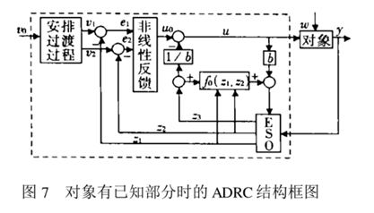
Its structure is divided into these parts, including transition process, non-linear feedback, extended state observer (ESO - Extended state observer), controlled object and so on. Next, it is explained one by one according to the citation 1 [1].
a. Arrangement of the transition process
Because the direct error method is not necessarily good, because e = r - y method is prone to overshoot, so for low disturbance - high precision control can not meet the requirements.
Therefore, a transition process v1(t) and v2(t) are arranged as differential signals, e = v1(t) - y is adopted, and the step response of the tracking differentiator is as follows: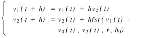
The variables h are step size, x1 and x2 are input vectors, r determines the following speed, h0 determines the filtering effect, and fst(v1,v2,h,r,h) is: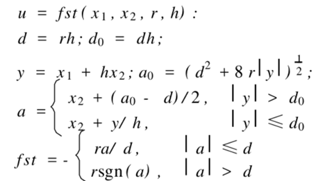
Among them, a, d and a0 are symbolic functions according to the parameters regulated by the system.
b. Extended State Observer (ESO)
Here is the extended state observer, where beta01, beta02, beta03, alpha1, alpha2., epsilon1 are all parameters, then the first derivative and z of z are state variables, where the fal function is: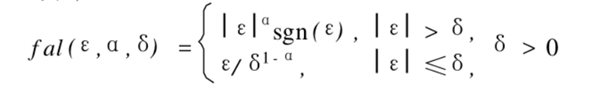
c. Nonlinear PID
Using tracking differentiator (TD), the classical PID is transformed into "non-linear PID", as shown in the figure.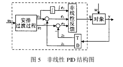
Here TD (Tracking Differentiator) gives the quantity z1 of tracking output y and its differential z2. Error, integral and differential are arranged transitional processes and TD.
The output z1, Z2 is generated.
The original "weighted sum" is replaced by "non-linear combination" to obtain "non-linear PID". The fal function mentioned above has the characteristics of small error, large gain, large error and small gain.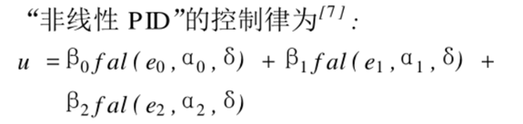
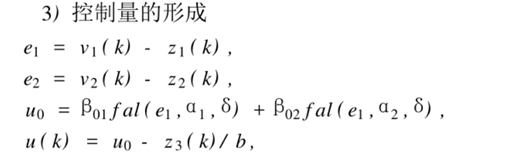
3.ADRC algorithm
Here is also a full use of Han Jingqing's algorithmic ideas to introduce, the above part is derived from the mathematics of continuous expressions, but we use discrete form in computer processing, or in real life applications. The following part is a screenshot of the discrete algorithm given by Mr. Han: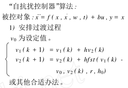


4.Matalb programming implementation and verification (this part is not perfect, I personally understand that only a part is completed, I hope someone can correct and discuss)
Here, the above content is entirely based on Mr. Han's paper. See Quoted Literature 1 for screenshot transcription, adding only a superficial self-understanding. The next part is the personal realization in matlab according to Mr. Han's thesis (whether it is correct or not is uncertain, I hope you can discuss and correct it). The annotations in it will be scrambled if they are opened again in Chinese, so we hope that we can not laugh at them with our own Chinglish annotations.
Code section:
a.fst function code implementation:
%%%
%Input Parameter:
%x1: Input vector1
%x2: Input vector2
%r : The speed of element;It up to tracking speed
%h : The filter of element;It determines the strength of filt.
%x : This is input vector.
%
%Output Parameter:
%y : Function output value.
%%%
function y = fst_function(x1,x2,r,h)

Length1 = length(x1);
% Length2 = length(x2);

% define the length of the variables.
% This can achieve smooth operation.
y = zeros(1,Length1);
a0 = zeros(1,Length1);
a = zeros(1,Length1);

% These two parameters are constants.
d  =  r*h;  % This parameter is known.
d0 =  d*h;  % Known.

  for i = 1:Length1
     % This part can get the value of three parameters.
     % get y a0 a,respectively.
     y(i)  =  x1(i) + h*x2(i);
     a0(i)  = power(d.^2 + 8*r*(abs(y(i))),1/2);
     if abs(y(i)) > d0
       a(i) = x2(i) + (a0(i) - d)./2;
     end
     if abs(y(i)) <= d0
       a(i) = x2(i) + y(i)./h;
     end

     %This is fst function.
     if abs(a(i)) <= d
        y(i) = -r*a(i)./d;
     end
     if abs(a(i)) > d
        y(i) = -r*sign(a(i));
     end
  end
end
Here is the fst_function function function of the FST function. The parameters are set randomly to check. The following is in the input section of the command windows window:
>> x1 = 0.1:0.2:10;
>> x2 = x1 + 0.01*rand;
>> r = 4;
>> h = 3;
>> y = fst_function(x1,x2,r,h);
>> plot(x1,y);
The results are as follows: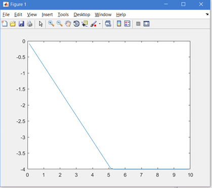
b.fal function implementation
%This function is fal function
%Input Parameter:
%alpha  : Parameter1
%delta  : Parameter2
%epsilon: Input Vector
%
%Output Parameter:
%y : Function output value.
%%%
function y = fal_function(alpha,delta,epsilon)

Length = length(epsilon);

% define the length of the variables.
% This can achieve smooth operation.
y = zeros(1,Length);

if delta <= 0
   error("Delta must greater than to zero");
end

for i = 1:Length

    if abs(epsilon(i)) > delta
       y(i) = (abs(epsilon(i)).^alpha)*sign(epsilon(i));
    end
    if abs(epsilon(i)) <= delta && delta > 0
       y(i) = epsilon(i)./(delta.^(1 - alpha));
    end

end
end
Here is the fal_function function function of the fst function, whose parameters are set randomly to check, as follows in the input section of the command windows window:
>> alpha = 3;
>> delta = 7;
>> epsilon = -19.9:0.1:20;
>> y = fal_function(alpha,delta,epsilon);
>> plot(epsilon,y);
The results are as follows:
c. According to the algorithm described above, the overall programming (not successful, I hope we can discuss it with you)
% TD + ESO + NLSEF = ADRC
function y = ADRC_Algorithm(Length)

% Call fst and fal function below.
fst = @fst_function;
fal = @fal_function;

% define the length of the variables.
% This can achieve smooth operation.
v1 = zeros(1,Length + 1);
v2 = zeros(1,Length + 1);
Z1 = zeros(1,Length + 1);
Z2 = zeros(1,Length + 1);
Z3 = zeros(1,Length + 1);
epsilon1 = zeros(1,Length + 1);
u0 = zeros(1,Length + 1);
e1 = zeros(1,Length + 1);
e2 = zeros(1,Length + 1);
u = zeros(1,Length + 1);

% Set System Parameters.
r = 0.1;      % r :Speed factor ;It depends on the tracking speed.
h0 = 4;       % h :Filter factor;It determines the strength of the filter.

% Set initial value.
v1(1) = 0.1;  % This is v1(0)
v2(1) = 0.2;  % This is v2(0)
Z1(1) = 0.5;  % This is Z1(0)
Z2(1) = 0.1;  % This is Z2(0)
Z3(1) = 0.7;  % This is Z3(0)
v0 = 8; %This is the Pro_Set or expectation value.(vital)

beta01 = 0.2;
beta02 = 0.3;
beta03 = 0.4;
b = 0.4;
delta = 3.5;

alpha1 = 0.5; %
alpha2 = 0.25; %

% Implemente algorithms and updates the data of parameters in the loop.
for i = 1:Length

    %Arrange the Transition Process
    v1(i+1) = v1(i) + h*v2(i);
    v2(i+1) = v2(i) + h*fst(v1(i) - v0,v2(k),r,h0);

    %Evaluate the state and total disturbance.
    %ESO Equation
    epsilon1(i) = Z1(i) - y(i);

    %f0(i) = z1(k) + z2(k);   %This function is known,but I don't know its expression.
    %u(i) = u0 - (z3(i) + f0(i))./b;

    %Control yolume formation
    u0(i) = beta01*fal(e1(i),a1pha1,delta) + beta02*fal(e2(i),alpha2,delta);
    u(i) = u0(i) + Z3(i)/b;

    Z1(i+1) = Z1(i) + h*(Z2(i) - beta01*epsilon1(i));
    Z2(i+1) = Z2(i) + h*(Z3(i) - beta02*fal(epsilon1(i),alpha1,delta)) + b*u(i);
    Z3(i+1) = Z3(i) - h*beta03*fal(epsilon1(i),alpha2,delta);

    %Control yolume formation
    e1(i) = v1(i) - Z1(i);
    e2(i) = v2(i) - Z2(i);

    %data update
    v1(i) = v1(i+1);
    v2(i) = v2(i+1);

    Z1(i) = Z1(i+1);
    Z2(i) = Z2(i+1);
    Z3(i) = Z3(i+1);

end
end

%This function is fst function
%%%
%Input Parameter:
%x1: Input vector1
%x2: Input vector2
%r : The speed of element;It up to tracking speed
%h : The filter of element;It determines the strength of filt.
%x : This is input vector.
%
%Output Parameter:
%y : Function output value.
%%%
function y = fst_function(x1,x2,r,h)

Length1 = length(x1);
% Length2 = length(x2);

% define the length of the variables.
% This can achieve smooth operation.
y = zeros(1,Length1);
a0 = zeros(1,Length1);
a = zeros(1,Length1);

% These two parameters are constants.
d  =  r*h;  % This parameter is known.
d0 =  d*h;  % Known.

  for i = 1:Length1
     % This part can get the value of three parameters.
     % get y a0 a,respectively.
     y(i)  =  x1(i) + h*x2(i);
     a0(i)  = power(d.^2 + 8*r*(abs(y(i))),1/2);
     if abs(y(i)) > d0
       a(i) = x2(i) + (a0(i) - d)./2;
     end
     if abs(y(i)) <= d0
       a(i) = x2(i) + y(i)./h;
     end

     %This is fst function.
     if abs(a(i)) <= d
        y(i) = -r*a(i)./d;
     end
     if abs(a(i)) > d
        y(i) = -r*sign(a(i));
     end
  end
end

%This function is fal function
%Input Parameter:
%alpha  : Input vector1
%delta  : Input vector2
%epsilon:
%
%Output Parameter:
%y : Function output value.
%%%
function y = fal_function(alpha,delta,epsilon)

Length = length(epsilon);

% define the length of the variables.
% This can achieve smooth operation.
y = zeros(1,Length);

if delta <= 0
   error("Delta must greater than to zero");
end

for i = 1:Length

    if abs(epsilon(i)) > delta
       y(i) = (abs(epsilon(i)).^alpha)*sign(epsilon(i));
    end
    if abs(epsilon(i)) <= delta && delta > 0
       y(i) = epsilon(i)./(delta.^(1 - alpha));
    end

end
end
Here, the problem is that the expression of f0 is not found in the paper, and a formula is added at will. There are also problems of parameter adjustment and initial value setting. All of these need to understand and add some practical projects in the next study to adjust to understand the meaning.
This is the beginning of learning, followed by the learning of PID understanding, as the beginning of understanding ADRC, this is my first blog, I will use my own understanding, after learning to share their results, and then we discuss progress together.
If there is any mention in the article, please comment on me if there is no source tagged. I will definitely add the source. If there is any infringement, please contact me and I will delete it as soon as possible.