Kinematics analysis of PUMA560
Reference textbook: Cai Zixing, the third edition of Robotics
PUMA560 modeling and simulation matlab code
matlab Toolbox: robotics toolbox
① Download address http://petercorke.com/wordpress/toolboxes/robotics-toolbox Download the installation package (. zip) format, and copy the extracted folder "rvctools" to the toolbox folder under the matlab installation path.
② Open matlab, click Set path - > > add and include subfolders, then select the "rvctools" folder, and finally save - > > close
③ Open the startup of the "rvctool" folder_ RVC. M runs, and the roboticstoolbox is installed. Or enter startup rvc on the matlab command line to install.
④ matlab command line input ver to see whether to install
>>ver
MATLAB edition: 9.5.0.944444 (R2018b)
Robotics Toolbox for MATLAB                           Version 10.3.1
Program description
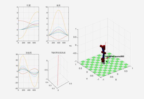
- According to the formula derivation in the textbook, four groups of solutions of the robot can be calculated, and then the other four groups of solutions can be obtained according to the "turnover" of wrist joint. (8 groups of solutions in total). In the process of planning, only one group of solutions is used, and the optimal solution is not selected. (the rest of the solutions have been commented out by me. If you are interested, you can try the other solutions 👏)
main program
% In trajectory planning, firstly, the robot model is established, 6 R Robot model, name modified puma560.
% Defining robots a--Connecting rod length, d--Connecting rod offset
	a2=0.4318;a3=0.02032;d2=0.14909;d4=0.43307;
%			 thetai    di      ai-1        alphai-1
    L1 = Link([pi/2    0       0               0], 'modified');
    L2 = Link([0       d2      0           -pi/2], 'modified');
    L3 = Link([-pi/2   0       a2              0], 'modified');
    L4 = Link([0       d4      a3          -pi/2], 'modified');
    L5 = Link([0       0  	   0            pi/2], 'modified');
    L6 = Link([0       0       0           -pi/2], 'modified');
    robot = SerialLink([L1,L2,L3,L4,L5,L6]);
    robot.name = 'modified puma560';
%   robot.display();
%	robot.teach();
% Define initial joint angle in trajectory planning( First_Theta)And end joint angle( Final_Theta),The number of steps is 777.
  % First_Theta = [0     pi/2  -pi/2   0       0     0];%Ready state
  % Final_Theta = [0     pi/4    pi    0       pi/4  0];%Dexterous state
% 6 Angle change
     First_Theta = [0     pi/2  -pi/2   0       0     0];
     Final_Theta = [pi/6  pi/4    pi    pi/3   pi/4  pi/2];
% jtraj Trajectory planning of function joint angle space
    step = 777;
    [q,qd,qdd] = jtraj(First_Theta,Final_Theta,step);

%The plane is divided into two*4=8 Sub drawing interval, a total of two lines, each line of four
%Position information of the first sub picture on the first line.
    subplot(2,4,1);
    i = 1:6;
    plot(q(:,i)); grid on;
    title('position');
%In the first line, the second sub picture speed information.
    subplot(2,4,2);
    i = 1:6;
    plot(qd(:,i));grid on;
    title('speed');
%In the second line, the first sub picture acceleration information.
    subplot(2,4,5);
    i = 1:6;
    plot(qdd(:,i));grid on;
    title('acceleration');

%according to First_Theta and Final_Theta The starting and ending pose matrices are obtained.
    %Using the self-contained function to solve
%     T0 = robot.fkine(First_Theta);
%     Tf = robot.fkine(Final_Theta);
    %According to the improvement DH The self-made function of the model, kinematics Forward kinematics solution
     T0=kinematics(First_Theta);
     T0=SE3(T0);
     Tf=kinematics(Final_Theta);
     Tf=SE3(Tf);
%utilize ctraj Planning trajectories in Cartesian space.
    Tc = ctraj(T0,Tf,step);
%The moving variable is extracted from the homogeneous rotation matrix, which is equivalent to the position of points in Cartesian coordinate system.
    Tjtraj = transl(Tc);
%On the second line, the second sub picture p1 reach p2 Straight track.
    subplot(2,4,6);
    plot2(Tjtraj,'r');grid on;
    title('T0 reach Tf Straight track');

%     hold on;
%Three or four subgraphs in the first row and three or four subgraphs in the second row are equivalent to drawing the entire right half
    subplot(2,4,[3,4,7,8]);

 for Var = 1:777
     T1=Tc(1,Var);
     T2=T1.T;
 % Inverse_kinematics Inverse kinematics solution
  qq(:,Var) = Inverse_kinematics(T2);
 end
 plot2(Tjtraj,'r');
 robot.plot(qq');
Kinematics function (forward kinematics)
function T0_6=kinematics(theta1_6)
    a2=0.4318;a3=0.02032;d2=0.14909;d4=0.43307;
	theta1=theta1_6(1);
	theta2=theta1_6(2);
	theta3=theta1_6(3);
	theta4=theta1_6(4);
	theta5=theta1_6(5);
	theta6=theta1_6(6);
	c1=cos(theta1);s1=sin(theta1);
	c2=cos(theta2);s2=sin(theta2);
	c3=cos(theta3);s3=sin(theta3);
	c4=cos(theta4);s4=sin(theta4);
	c5=cos(theta5);s5=sin(theta5);
	c6=cos(theta6);s6=sin(theta6);
	%6 Transformation matrix of connecting rod
    T1=[c1 -s1 0 0;s1 c1 0 0;0 0 1 0;0 0 0 1];
    T2=[c2 -s2 0 0;0 0 1 d2;-s2 -c2 0 0;0 0 0 1];
    T3=[c3 -s3 0 a2;s3 c3 0 0 ;0 0 1 0;0 0 0 1];
    T4=[c4 -s4 0 a3;0 0 1 d4;-s4 -c4 0 0;0 0 0 1];
    T5=[c5 -s5 0 0 ;0 0 -1 0;s5 c5 0 0;0 0 0 1];
    T6=[c6 -s6 0 0 ;0 0 1 0;-s6 -c6 0 0;0 0 0 1];
    %Forward kinematics equation
    T0_6 = T1*T2*T3*T4*T5*T6;
end
Inverse_kinematics function (inverse kinematics)
function theta_Med=Inverse_kinematics(T)
% a--Connecting rod length, d--Connecting rod offset
	a2=0.4318;a3=0.02032;d2=0.14909;d4=0.43307;

     nx=T(1,1); ny=T(2,1); nz=T(3,1);
     ox=T(1,2); oy=T(2,2); oz=T(3,2);
     ax=T(1,3); ay=T(2,3); az=T(3,3);
     px=T(1,4); py=T(2,4); pz=T(3,4);

% For the convenience of calculation, the m Series vector
% Solving joint angle 1
	theta1_1 = atan2(py,px)-atan2(d2,sqrt(px^2+py^2-d2^2));
	theta1_2 = atan2(py,px)-atan2(d2,-sqrt(px^2+py^2-d2^2));
% Solving joint angle 3
	m3_1 = (px^2+py^2+pz^2-a2^2-a3^2-d2^2-d4^2)/(2*a2);
	theta3_1 = atan2(a3,d4)-atan2(m3_1,sqrt(a3^2+d4^2-m3_1^2));
	theta3_2 = atan2(a3,d4)-atan2(m3_1,-sqrt(a3^2+d4^2-m3_1^2));
% Solving joint angle 2
    ms2_1 = -((a3+a2*cos(theta3_1))*pz)+(cos(theta1_1)*px+sin(theta1_1)*py)*...
    (a2*sin(theta3_1)-d4);
    mc2_1 = (-d4+a2*sin(theta3_1))*pz+(cos(theta1_1)*px+sin(theta1_1)*py)*...
    (a2*cos(theta3_1)+a3);
    theta23_1 = atan2(ms2_1,mc2_1);
    theta2_1 = theta23_1 - theta3_1;

    ms2_2 = -((a3+a2*cos(theta3_1))*pz)+(cos(theta1_2)*px+sin(theta1_2)*py)*...
    (a2*sin(theta3_1)-d4);
    mc2_2 = (-d4+a2*sin(theta3_1))*pz+(cos(theta1_2)*px+sin(theta1_2)*py)*...
    (a2*cos(theta3_1)+a3);
    theta23_2 = atan2(ms2_2,mc2_2);
    theta2_2 = theta23_2 - theta3_1;

    ms2_3 = -((a3+a2*cos(theta3_2))*pz)+(cos(theta1_1)*px+sin(theta1_1)*py)*...
    (a2*sin(theta3_2)-d4);
    mc2_3 = (-d4+a2*sin(theta3_2))*pz+(cos(theta1_1)*px+sin(theta1_1)*py)*...
    (a2*cos(theta3_2)+a3);
    theta23_3 = atan2(ms2_3,mc2_3);
    theta2_3 = theta23_3 - theta3_2;


    ms2_4 = -((a3+a2*cos(theta3_2))*pz)+(cos(theta1_2)*px+sin(theta1_2)*py)*...
    (a2*sin(theta3_2)-d4);
    mc2_4 = (-d4+a2*sin(theta3_2))*pz+(cos(theta1_2)*px+sin(theta1_2)*py)*...
    (a2*cos(theta3_2)+a3);
    theta23_4 = atan2(ms2_4,mc2_4);
    theta2_4 = theta23_4 - theta3_2;
% Solving joint angle 4
    ms4_1=-ax*sin(theta1_1)+ay*cos(theta1_1);
    mc4_1=-ax*cos(theta1_1)*cos(theta23_1)-ay*sin(theta1_1)*...
    cos(theta23_1)+az*sin(theta23_1);
	theta4_1=atan2(ms4_1,mc4_1);

	ms4_2=-ax*sin(theta1_2)+ay*cos(theta1_2);
    mc4_2=-ax*cos(theta1_2)*cos(theta23_2)-ay*sin(theta1_2)*...
    cos(theta23_2)+az*sin(theta23_2);
	theta4_2=atan2(ms4_2,mc4_2);

	ms4_3=-ax*sin(theta1_1)+ay*cos(theta1_1);
    mc4_3=-ax*cos(theta1_1)*cos(theta23_3)-ay*sin(theta1_1)*...
    cos(theta23_3)+az*sin(theta23_3);
	theta4_3=atan2(ms4_3,mc4_3);

	ms4_4=-ax*sin(theta1_2)+ay*cos(theta1_2);
    mc4_4=-ax*cos(theta1_2)*cos(theta23_4)-ay*sin(theta1_2)*...
    cos(theta23_4)+az*sin(theta23_4);
	theta4_4=atan2(ms4_4,mc4_4);
% Solving joint angle 5
	ms5_1=-ax*(cos(theta1_1)*cos(theta23_1)*cos(theta4_1)+...
	sin(theta1_1)*sin(theta4_1))-...
	ay*(sin(theta1_1)*cos(theta23_1)*cos(theta4_1)-cos(theta1_1)*sin(theta4_1))...
    +az*(sin(theta23_1)*cos(theta4_1));
    mc5_1= ax*(-cos(theta1_1)*sin(theta23_1))+ay*(-sin(theta1_1)*sin(theta23_1))...
           +az*(-cos(theta23_1));
    theta5_1=atan2(ms5_1,mc5_1);

	ms5_2=-ax*(cos(theta1_2)*cos(theta23_2)*cos(theta4_2)+...
	sin(theta1_2)*sin(theta4_2))-...
	ay*(sin(theta1_2)*cos(theta23_2)*cos(theta4_2)-cos(theta1_2)*sin(theta4_2))...
    +az*(sin(theta23_2)*cos(theta4_2));
    mc5_2= ax*(-cos(theta1_2)*sin(theta23_2))+ay*(-sin(theta1_2)*sin(theta23_2))...
           +az*(-cos(theta23_2));
    theta5_2=atan2(ms5_2,mc5_2);

	ms5_3=-ax*(cos(theta1_1)*cos(theta23_3)*cos(theta4_3)+...
	sin(theta1_1)*sin(theta4_3))-...
	ay*(sin(theta1_1)*cos(theta23_3)*cos(theta4_3)-cos(theta1_1)*sin(theta4_3))...
    +az*(sin(theta23_3)*cos(theta4_3));
    mc5_3= ax*(-cos(theta1_1)*sin(theta23_3))+ay*(-sin(theta1_1)*sin(theta23_3))...
           +az*(-cos(theta23_3));
    theta5_3=atan2(ms5_3,mc5_3);

	ms5_4=-ax*(cos(theta1_2)*cos(theta23_4)*cos(theta4_4)+...
	sin(theta1_2)*sin(theta4_4))-...
	ay*(sin(theta1_2)*cos(theta23_4)*cos(theta4_4)-cos(theta1_2)*sin(theta4_4))...
    +az*(sin(theta23_4)*cos(theta4_4));
    mc5_4= ax*(-cos(theta1_2)*sin(theta23_4))+ay*(-sin(theta1_2)*sin(theta23_4))...
           +az*(-cos(theta23_4));
    theta5_4=atan2(ms5_4,mc5_4);
% Solving joint angle 6
	ms6_1=-nx*(cos(theta1_1)*cos(theta23_1)*...
			sin(theta4_1)-sin(theta1_1)*cos(theta4_1))...
        -ny*(sin(theta1_1)*cos(theta23_1)*...
        	sin(theta4_1)+cos(theta1_1)*cos(theta4_1))...
        +nz*(sin(theta23_1)*sin(theta4_1));
    mc6_1= nx*(cos(theta1_1)*cos(theta23_1)*cos(theta4_1)...
         +sin(theta1_1)*sin(theta4_1))*cos(theta5_1)...
         -nx*cos(theta1_1)*sin(theta23_1)*sin(theta4_1)...
         +ny*(sin(theta1_1)*cos(theta23_1)*cos(theta4_1)...
        +cos(theta1_1)*sin(theta4_1))*cos(theta5_1)...
        -ny*sin(theta1_1)*sin(theta23_1)*sin(theta5_1)...
        -nz*(sin(theta23_1)*cos(theta4_1)*cos(theta5_1)...
        +cos(theta23_1)*sin(theta5_1));
	theta6_1=atan2(ms6_1,mc6_1);

	ms6_2=-nx*(cos(theta1_2)*cos(theta23_2)*...
			sin(theta4_2)-sin(theta1_2)*cos(theta4_2))...
        -ny*(sin(theta1_2)*cos(theta23_2)*...
        	sin(theta4_2)+cos(theta1_2)*cos(theta4_2))...
        +nz*(sin(theta23_2)*sin(theta4_2));
    mc6_2= nx*(cos(theta1_2)*cos(theta23_2)*cos(theta4_2)...
         +sin(theta1_2)*sin(theta4_2))*cos(theta5_2)...
         -nx*cos(theta1_2)*sin(theta23_2)*sin(theta4_2)...
         +ny*(sin(theta1_2)*cos(theta23_2)*cos(theta4_2)...
        +cos(theta1_2)*sin(theta4_2))*cos(theta5_2)...
        -ny*sin(theta1_2)*sin(theta23_2)*sin(theta5_2)...
        -nz*(sin(theta23_2)*cos(theta4_2)*cos(theta5_2)...
        +cos(theta23_2)*sin(theta5_2));
	theta6_2=atan2(ms6_2,mc6_2);

	ms6_3=-nx*(cos(theta1_1)*cos(theta23_3)*...
			sin(theta4_3)-sin(theta1_1)*cos(theta4_3))...
        -ny*(sin(theta1_1)*cos(theta23_3)*...
        	sin(theta4_3)+cos(theta1_1)*cos(theta4_3))...
        +nz*(sin(theta23_3)*sin(theta4_3));
    mc6_3= nx*(cos(theta1_1)*cos(theta23_3)*cos(theta4_3)...
         +sin(theta1_1)*sin(theta4_3))*cos(theta5_3)...
         -nx*cos(theta1_1)*sin(theta23_3)*sin(theta4_3)...
         +ny*(sin(theta1_1)*cos(theta23_3)*cos(theta4_3)...
        +cos(theta1_1)*sin(theta4_3))*cos(theta5_3)...
        -ny*sin(theta1_1)*sin(theta23_3)*sin(theta5_3)...
        -nz*(sin(theta23_3)*cos(theta4_3)*cos(theta5_3)...
        +cos(theta23_3)*sin(theta5_3));
	theta6_3=atan2(ms6_3,mc6_3);

	ms6_4=-nx*(cos(theta1_2)*cos(theta23_4)*...
			sin(theta4_4)-sin(theta1_2)*cos(theta4_4))...
        -ny*(sin(theta1_1)*cos(theta23_4)*...
        	sin(theta4_4)+cos(theta1_2)*cos(theta4_4))...
        +nz*(sin(theta23_4)*sin(theta4_4));
    mc6_4= nx*(cos(theta1_2)*cos(theta23_4)*cos(theta4_4)...
         +sin(theta1_2)*sin(theta4_4))*cos(theta5_4)...
         -nx*cos(theta1_2)*sin(theta23_4)*sin(theta4_4)...
         +ny*(sin(theta1_2)*cos(theta23_4)*cos(theta4_4)...
        +cos(theta1_2)*sin(theta4_4))*cos(theta5_1)...
        -ny*sin(theta1_2)*sin(theta23_4)*sin(theta5_4)...
        -nz*(sin(theta23_4)*cos(theta4_4)*cos(theta5_4)...
        +cos(theta23_4)*sin(theta5_4));
	theta6_4=atan2(ms6_4,mc6_4);


% Four groups of nonsingular inverse kinematics solutions are obtained
	theta_Med_1 = [ theta1_1,theta2_1,theta3_1,theta4_1,theta5_1,theta6_1;
				   %theta1_2,theta2_2,theta3_1,theta4_2,theta5_2,theta6_2;
				   %theta1_1,theta2_3,theta3_2,theta4_3,theta5_3,theta6_3;
				   %theta1_2,theta2_4,theta3_2,theta4_4,theta5_4,theta6_4;
                 ];
% The joint will be manipulated'Flip'Four other groups of solutions can be obtained
theta_Med_2 = ...
    [ %theta1_1,theta2_1,theta3_1,theta4_1+pi,-theta5_1,theta6_1+pi;
	  %theta1_2,theta2_2,theta3_1,theta4_2+pi,-theta5_2,theta6_2+pi;
	  %theta1_1,theta2_3,theta3_2,theta4_3+pi,-theta5_3,theta6_3+pi;
	  %theta1_2,theta2_4,theta3_2,theta4_4+pi,-theta5_4,theta6_4+pi;
      ];
  theta_Med=[theta_Med_1;theta_Med_2];
end
Operation results
