After installing Tensorflow, install keras to use TF as the back-end by default. The code of keras to realize convolution network is very simple, and the callback class in keras provides a method to detect variables in the model training process, which can adjust the learning efficiency and some parameters of the model in time according to the situation of detecting variables. In the following example, MNIST data is used as the test
import pandas as pd
import numpy as np
import matplotlib.pyplot as plt
import matplotlib.image as pimg
import seaborn as sb         # A painting module based on matplotlib, supporting numpy,pandas and other data structures
%matplotlib inline

from sklearn.model_selection import train_test_split
from sklearn.metrics import confusion_matrix     # Confusion matrix

import itertools
#  keras
from keras.utils import to_categorical         #Digital tag transformed into one-hot code
from keras.models import Sequential
from keras.layers import Dense,Dropout,Flatten,Conv2D,MaxPool2D
from keras.optimizers import RMSprop
from keras.preprocessing.image import ImageDataGenerator
from keras.callbacks import ReduceLROnPlateau
Using TensorFlow backend.
# Set painting style
sb.set(style='white', context='notebook', palette='deep')
# Loading data
train_data = pd.read_csv('data/train.csv')
test_data = pd.read_csv('data/test.csv')
#train_x = train_data.drop(labels=['label'],axis=1)  # Remove label column
train_x = train_data.iloc[:,1:]
train_y = train_data.iloc[:,0]
del  train_data   # Free up some memory
# Observe the distribution of training data
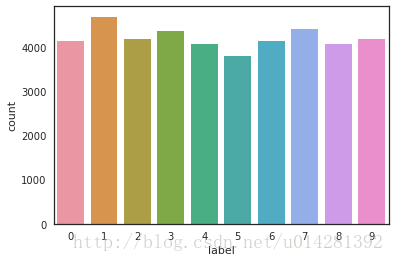
g = sb.countplot(train_y)
train_y.value_counts()
1    4684
7    4401
3    4351
9    4188
2    4177
6    4137
0    4132
4    4072
8    4063
5    3795
Name: label, dtype: int64

train_x.isnull().describe() # Check for a true value
train_x.isnull().any().describe()
count       784
unique        1
top       False
freq        784
dtype: object
test_data.isnull().any().describe()
count       784
unique        1
top       False
freq        784
dtype: object
# normalization
train_x =  train_x/255.0
test_x = test_data/255.0
del test_data
Transform the shape of data
# reshape trian_x, test_x
#train_x = train_x.values.reshape(-1, 28, 28, 1)
#test_x = test_x.values.reshape(-1, 28, 28, 1)
train_x = train_x.as_matrix().reshape(-1, 28, 28, 1)
test_x = test_x.as_matrix().reshape(-1, 28, 28, 1)
# Convert the label column to one hot encoding format
train_y = to_categorical(train_y, num_classes = 10)
Separate validation data from data
#One tenth of training data is used as verification data
random_seed = 3
train_x , val_x , train_y, val_y = train_test_split(train_x, train_y, test_size=0.1, random_state=random_seed)
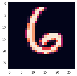
A training sample
plt.imshow(train_x[0][:,:,0])

Building CNN with Keras
model = Sequential()
# First convolution layer, 32 convolution kernels, size 5x5, convolution mode save, activation function relu, input tensor size
model.add(Conv2D(filters= 32, kernel_size=(5,5), padding='Same', activation='relu',input_shape=(28,28,1)))
model.add(Conv2D(filters= 32, kernel_size=(5,5), padding='Same', activation='relu'))
# Pool layer, pool core size 2x2
model.add(MaxPool2D(pool_size=(2,2)))
# Randomly discard one quarter of network connections to prevent over fitting
model.add(Dropout(0.25))
model.add(Conv2D(filters= 64, kernel_size=(3,3), padding='Same', activation='relu'))
model.add(Conv2D(filters= 64, kernel_size=(3,3), padding='Same', activation='relu'))
model.add(MaxPool2D(pool_size=(2,2), strides=(2,2)))
model.add(Dropout(0.25))
# Full connection layer, expand operation,
model.add(Flatten())
# Add the number of hidden layer neurons and activation function
model.add(Dense(256, activation='relu'))
model.add(Dropout(0.25))
# Output layer
model.add(Dense(10, activation='softmax'))
# Set optimizer
# lr: learning efficiency, decay: attenuation value of lr
optimizer = RMSprop(lr = 0.001, decay=0.0)
# Compilation model
# Loss: loss function, metrics: corresponding performance evaluation function
model.compile(optimizer=optimizer, loss = 'categorical_crossentropy',metrics=['accuracy'])
Create an instance of the callback class
# The callback class of keras provides the ability to track target values and dynamically adjust learning efficiency
# Monitor: the quantity to be monitored, here is the verification accuracy rate
# Animation: after three rounds of iterations, the target amount of monitoring is still unchanged, and the learning efficiency will be adjusted
# verbose: information display mode, to 0 or 1
# Factor: each time the learning rate is reduced, the learning rate will be reduced in the form of lr = lr*factor
# Mode: "auto", "min", "max". In min mode, if the detection value triggers the decrease of learning rate. In max mode, when the detection value no longer increases, the learning rate decreases.
# epsilon: threshold value used to determine whether to enter the "plain area" of the detection value
# Cooldown: after the learning rate is reduced, normal operation will be resumed after cooldown epoch s
# Min? LR: the lower limit of learning rate
learning_rate_reduction = ReduceLROnPlateau(monitor = 'val_acc', patience = 3,
                                            verbose = 1, factor=0.5, min_lr = 0.00001)
epochs = 40
batch_size = 100
Data enhancement processing
# Data enhancement processing can improve the generalization ability of the model, and also can effectively avoid the over fitting of the model
# Rotation? Range: angle of rotation
# Zoom range: randomly scale an image
# Width? Shift? Range: ratio of horizontal movement to image width
# height_shift_range
# Horizontal inverted
# Vertical? FILP: reverse in the vertical direction
data_augment = ImageDataGenerator(rotation_range= 10,zoom_range= 0.1,
                                  width_shift_range = 0.1,height_shift_range = 0.1,
                                  horizontal_flip = False, vertical_flip = False)
Training model
history = model.fit_generator(data_augment.flow(train_x, train_y, batch_size=batch_size),
                             epochs= epochs, validation_data = (val_x,val_y),
                             verbose =2, steps_per_epoch=train_x.shape[0]//batch_size,
                             callbacks=[learning_rate_reduction])
Epoch 1/40
359s - loss: 0.4529 - acc: 0.8498 - val_loss: 0.0658 - val_acc: 0.9793
Epoch 2/40
375s - loss: 0.1188 - acc: 0.9637 - val_loss: 0.0456 - val_acc: 0.9848
Epoch 3/40
374s - loss: 0.0880 - acc: 0.9734 - val_loss: 0.0502 - val_acc: 0.9845
Epoch 4/40
375s - loss: 0.0750 - acc: 0.9767 - val_loss: 0.0318 - val_acc: 0.9902
Epoch 5/40
374s - loss: 0.0680 - acc: 0.9800 - val_loss: 0.0379 - val_acc: 0.9888
Epoch 6/40
369s - loss: 0.0584 - acc: 0.9823 - val_loss: 0.0267 - val_acc: 0.9910
Epoch 7/40
381s - loss: 0.0556 - acc: 0.9832 - val_loss: 0.0505 - val_acc: 0.9824
Epoch 8/40
381s - loss: 0.0531 - acc: 0.9842 - val_loss: 0.0236 - val_acc: 0.9912
Epoch 9/40
376s - loss: 0.0534 - acc: 0.9839 - val_loss: 0.0310 - val_acc: 0.9910
Epoch 10/40
379s - loss: 0.0537 - acc: 0.9848 - val_loss: 0.0274 - val_acc: 0.9917
Epoch 11/40
375s - loss: 0.0501 - acc: 0.9856 - val_loss: 0.0254 - val_acc: 0.9931
Epoch 12/40
382s - loss: 0.0492 - acc: 0.9860 - val_loss: 0.0212 - val_acc: 0.9924
Epoch 13/40
380s - loss: 0.0482 - acc: 0.9864 - val_loss: 0.0259 - val_acc: 0.9919
Epoch 14/40
373s - loss: 0.0488 - acc: 0.9858 - val_loss: 0.0305 - val_acc: 0.9905
Epoch 15/40

Epoch 00014: reducing learning rate to 0.000500000023749.
370s - loss: 0.0493 - acc: 0.9853 - val_loss: 0.0259 - val_acc: 0.9919
Epoch 16/40
367s - loss: 0.0382 - acc: 0.9888 - val_loss: 0.0176 - val_acc: 0.9936
Epoch 17/40
376s - loss: 0.0376 - acc: 0.9891 - val_loss: 0.0187 - val_acc: 0.9945
Epoch 18/40
376s - loss: 0.0410 - acc: 0.9885 - val_loss: 0.0220 - val_acc: 0.9926
Epoch 19/40
371s - loss: 0.0385 - acc: 0.9886 - val_loss: 0.0194 - val_acc: 0.9933
Epoch 20/40
372s - loss: 0.0345 - acc: 0.9894 - val_loss: 0.0186 - val_acc: 0.9938
Epoch 21/40

Epoch 00020: reducing learning rate to 0.000250000011874.
375s - loss: 0.0395 - acc: 0.9888 - val_loss: 0.0233 - val_acc: 0.9945
Epoch 22/40
369s - loss: 0.0313 - acc: 0.9907 - val_loss: 0.0141 - val_acc: 0.9955
Epoch 23/40
376s - loss: 0.0308 - acc: 0.9910 - val_loss: 0.0187 - val_acc: 0.9945
Epoch 24/40
374s - loss: 0.0331 - acc: 0.9908 - val_loss: 0.0170 - val_acc: 0.9940
Epoch 25/40
372s - loss: 0.0325 - acc: 0.9904 - val_loss: 0.0166 - val_acc: 0.9948
Epoch 26/40

Epoch 00025: reducing learning rate to 0.000125000005937.
373s - loss: 0.0319 - acc: 0.9904 - val_loss: 0.0167 - val_acc: 0.9943
Epoch 27/40
372s - loss: 0.0285 - acc: 0.9915 - val_loss: 0.0138 - val_acc: 0.9950
Epoch 28/40
375s - loss: 0.0280 - acc: 0.9913 - val_loss: 0.0150 - val_acc: 0.9950
Epoch 29/40

Epoch 00028: reducing learning rate to 6.25000029686e-05.
377s - loss: 0.0281 - acc: 0.9924 - val_loss: 0.0158 - val_acc: 0.9948
Epoch 30/40
374s - loss: 0.0265 - acc: 0.9920 - val_loss: 0.0134 - val_acc: 0.9952
Epoch 31/40
378s - loss: 0.0270 - acc: 0.9922 - val_loss: 0.0128 - val_acc: 0.9957
Epoch 32/40
372s - loss: 0.0237 - acc: 0.9930 - val_loss: 0.0133 - val_acc: 0.9957
Epoch 33/40
375s - loss: 0.0237 - acc: 0.9931 - val_loss: 0.0138 - val_acc: 0.9955
Epoch 34/40
371s - loss: 0.0276 - acc: 0.9920 - val_loss: 0.0135 - val_acc: 0.9962
Epoch 35/40
373s - loss: 0.0259 - acc: 0.9920 - val_loss: 0.0136 - val_acc: 0.9952
Epoch 36/40
369s - loss: 0.0249 - acc: 0.9924 - val_loss: 0.0126 - val_acc: 0.9952
Epoch 37/40
370s - loss: 0.0257 - acc: 0.9923 - val_loss: 0.0130 - val_acc: 0.9960
Epoch 38/40

Epoch 00037: reducing learning rate to 3.12500014843e-05.
374s - loss: 0.0252 - acc: 0.9926 - val_loss: 0.0136 - val_acc: 0.9950
Epoch 39/40
372s - loss: 0.0246 - acc: 0.9927 - val_loss: 0.0134 - val_acc: 0.9957
Epoch 40/40
371s - loss: 0.0247 - acc: 0.9929 - val_loss: 0.0139 - val_acc: 0.9950
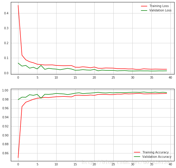
In the process of training, there are several conditions that trigger the learning efficiency decay. When val'acc does not increase for three consecutive rounds, it will adjust the learning efficiency to the current half. After the adjustment, val'acc has a significant increase, but in the last few rounds, the model may have converged
# learning curves
fig,ax = plt.subplots(2,1,figsize=(10,10))
ax[0].plot(history.history['loss'], color='r', label='Training Loss')
ax[0].plot(history.history['val_loss'], color='g', label='Validation Loss')
ax[0].legend(loc='best',shadow=True)
ax[0].grid(True)


ax[1].plot(history.history['acc'], color='r', label='Training Accuracy')
ax[1].plot(history.history['val_acc'], color='g', label='Validation Accuracy')
ax[1].legend(loc='best',shadow=True)
ax[1].grid(True)

# Confusion matrix
def plot_sonfusion_matrix(cm, classes, normalize=False, title='Confusion matrix',cmap=plt.cm.Blues):
    plt.imshow(cm, interpolation='nearest', cmap=cmap)
    plt.title(title)
    plt.colorbar()
    tick_marks = np.arange(len(classes))
    plt.xticks(tick_marks, classes, rotation=45)
    plt.yticks(tick_marks, classes)
    if normalize:
        cm = cm.astype('float')/cm.sum(axis=1)[:,np.newaxis]
    thresh = cm.max()/2.0
    for i,j in itertools.product(range(cm.shape[0]), range(cm.shape[1])):
        plt.text(j,i,cm[i,j], horizontalalignment='center',color='white' if cm[i,j] > thresh else 'black')
    plt.tight_layout()
    plt.ylabel('True label')
    plt.xlabel('Predict label')
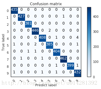
Confusing proof of validation data
pred_y = model.predict(val_x)
pred_label = np.argmax(pred_y, axis=1)
true_label = np.argmax(val_y, axis=1)

confusion_mat = confusion_matrix(true_label, pred_label)

plot_sonfusion_matrix(confusion_mat, classes = range(10))


