Kalman filter for tracking and prediction of moving targets on images
brief introduction
-
Kalman filter predicts the current state through the previous state and uses the current observation state for correction
-
The direct measurements are left, top, right and bottom, representing the upper left and lower right coordinates of the target respectively
-
It is generally believed that the speed of motion is uniform
-
However, the camera depression angle in the monitoring scene is too large and there is depth of field, resulting in non-uniform motion
- Come and go, from far to near, accelerate the movement
- Direction, from near to far, slow down
-
For non-uniform speed
- Target state quantity introduces acceleration
- The target state goes to the world coordinate system
- Binocular or multi camera: directly obtain the three-dimensional coordinates of the target in the camera coordinate system
- Monocular can be transferred to the world coordinate system by homography transformation matrix
-
Select the coming vehicle, obtain 53 frame motion coordinates, select the first 43 frames for prediction update, and the last 10 frames for prediction experiment

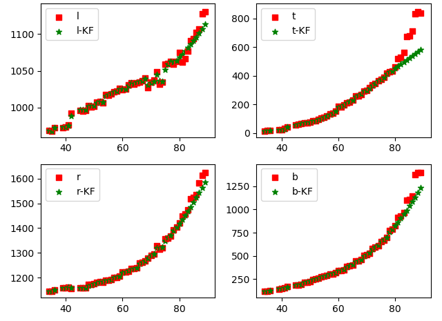
Uniform motion model
- State quantity: l , t , r , b , v l , v t , v r , v b l,t,r,b, v_l, v_t, v_r, v_b l. T, R, B, VL, vt, vr and vb are the position and corresponding velocity of the upper left corner and the lower right corner respectively
- Observation and measurement: l , t , r , b l,t,r,b l,t,r,b
- Uniform motion of object
- Tracking discontinuous frames
- The observation noise variance is related to the process noise error and the bbox height. The larger the h is, the larger the error is, and it can be updated in real time
class KalmanFilter:
    def __init__(self):
        self._std_weight_pos = 1. / 20     # position
        self._std_weight_vel = 1. / 160    # speed
        self.H = np.matrix(np.zeros((4, 8)))  # Observation matrix Z_t = Hx_t + v
        for i in range(4):
            self.H[i, i] = 1
        self.F = np.matrix(np.eye(8)) # State transition matrix

    def init(self, val):
        l,t,r,b = val
        mean_pos = np.matrix([[l], [t], [r], [b]])
        mean_vel = np.zeros_like(mean_pos) # Speed initialized to 0
        self.x_hat = np.r_[mean_pos, mean_vel] # x_k = [p, v]
        h = b - t
        std_pos = [
            2 * self._std_weight_pos * h,
            2 * self._std_weight_pos * h,
            2 * self._std_weight_pos * h,
            2 * self._std_weight_pos * h]
        std_vel = [
            10 * self._std_weight_vel * h,
            10 * self._std_weight_vel * h,
            10 * self._std_weight_vel * h,
            10 * self._std_weight_vel * h]
        self.P = np.diag(np.square(np.r_[std_pos, std_vel])) # State covariance matrix

    def predict(self, delt_t, val=None):
        if val is not None:
            h = val[3] - val[1]
            std_pos = [
                self._std_weight_pos * h,
                self._std_weight_pos * h,
                self._std_weight_pos * h,
                self._std_weight_pos * h]
            std_vel = [
                self._std_weight_vel * h,
                self._std_weight_vel * h,
                self._std_weight_vel * h,
                self._std_weight_vel * h]
            self.Q = np.diag(np.square(np.r_[std_pos, std_vel])) # Real time change of process noise
        for i in range(4):
            self.F[i, i+4] = delt_t
        self.x_hat_minus = self.F * self.x_hat
        self.P_minus = self.F * self.P * self.F.T + self.Q

    def update(self, val):
        l,t,r,b = val
        h = b - t
        std_pos = [
            self._std_weight_pos * h,
            self._std_weight_pos * h,
            self._std_weight_pos * h,
            self._std_weight_pos * h]
        self.R = np.diag(np.square(std_pos)) # Observation noise variance
        measure = np.matrix([[l], [t], [r], [b]])
        self.K = self.P_minus * self.H.T * np.linalg.inv(self.H * self.P_minus * self.H.T + self.R)
        self.x_hat = self.x_hat_minus + self.K * (measure - self.H * self.x_hat_minus)
        self.P = self.P_minus - self.K * self.H * self.P_minus
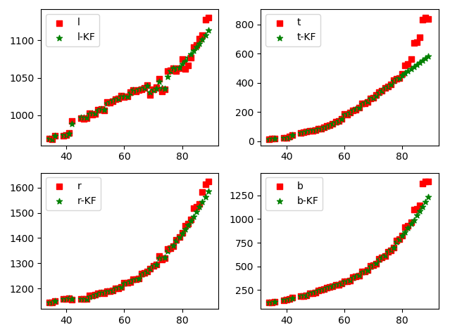
Introduction acceleration
- State quantity: l , t , r , b , v l , v t , v r , v b , a l , a t , a r , a b l,t,r,b,v_l, v_t,v_r,v_b,a_l,a_t,a_r,a_b l,t,r,b,vl,vt,vr,vb,al,at,ar,ab
- Observation and measurement: l , t , r , b l,t,r,b l,t,r,b
- Accelerated motion of object
- Tracking discontinuous frames
- The observation noise variance is related to the process noise error and the bbox height. The larger the h is, the larger the error is, and it can be updated in real time
class KalmanFilter2:
    def __init__(self):
        self._std_weight_pos = 1. / 20     # position
        self._std_weight_vel = 1. / 160    # speed
        self._std_weight_acc = 1. / 300    # speed
        self.H = np.matrix(np.zeros((4, 12)))  # Observation matrix Z_t = Hx_t + v
        for i in range(4):
            self.H[i, i] = 1
        self.F = np.matrix(np.eye(12))  # State transition matrix

    def init(self, val):
        l,t,r,b = val
        mean_pos = np.matrix([[l], [t], [r], [b]])
        mean_vel = np.zeros_like(mean_pos) # Speed initialized to 0
        mean_acc = np.zeros_like(mean_pos) # Speed initialized to 0
        self.x_hat = np.r_[mean_pos, mean_vel, mean_acc] # x_k = [p, v]
        h = b - t
        std_pos = [
            2 * self._std_weight_pos * h,
            2 * self._std_weight_pos * h,
            2 * self._std_weight_pos * h,
            2 * self._std_weight_pos * h]
        std_vel = [
            10 * self._std_weight_vel * h,
            10 * self._std_weight_vel * h,
            10 * self._std_weight_vel * h,
            10 * self._std_weight_vel * h]
        std_acc = [
            50 * self._std_weight_acc * h,
            50 * self._std_weight_acc * h,
            50 * self._std_weight_acc * h,
            50 * self._std_weight_acc * h
        ]
        self.P = np.diag(np.square(np.r_[std_pos, std_vel, std_acc])) # State covariance matrix

    def predict(self, delt_t, val=None):
        if val is not None:
            l,t,r,b = val
            h = b - t
            std_pos = [
                self._std_weight_pos * h,
                self._std_weight_pos * h,
                self._std_weight_pos * h,
                self._std_weight_pos * h]
            std_vel = [
                self._std_weight_vel * h,
                self._std_weight_vel * h,
                self._std_weight_vel * h,
                self._std_weight_vel * h]
            std_acc = [
                self._std_weight_acc * h,
                self._std_weight_acc * h,
                self._std_weight_acc * h,
                self._std_weight_acc * h]
            self.Q = np.diag(np.square(np.r_[std_pos, std_vel, std_acc])) # Real time change of process noise
        for i in range(4):
            self.F[i,i + 4] = delt_t
            self.F[i,i + 8] = delt_t ** 2 / 2
        for i in range(4, 8):
            self.F[i,i+4] = delt_t
        self.x_hat_minus = self.F * self.x_hat
        self.P_minus = self.F * self.P * self.F.T + self.Q

    def update(self, val):
        l,t,r,b = val
        h = b - t
        std_pos = [
            self._std_weight_pos * h,
            self._std_weight_pos * h,
            self._std_weight_pos * h,
            self._std_weight_pos * h]
        self.R = np.diag(np.square(std_pos)) # Observation noise variance
        measure = np.matrix([[l], [t], [r], [b]])
        self.K = self.P_minus * self.H.T * np.linalg.inv(self.H * self.P_minus * self.H.T + self.R)
        self.x_hat = self.x_hat_minus + self.K * (measure - self.H * self.x_hat_minus)
        self.P = self.P_minus - self.K * self.H * self.P_minus
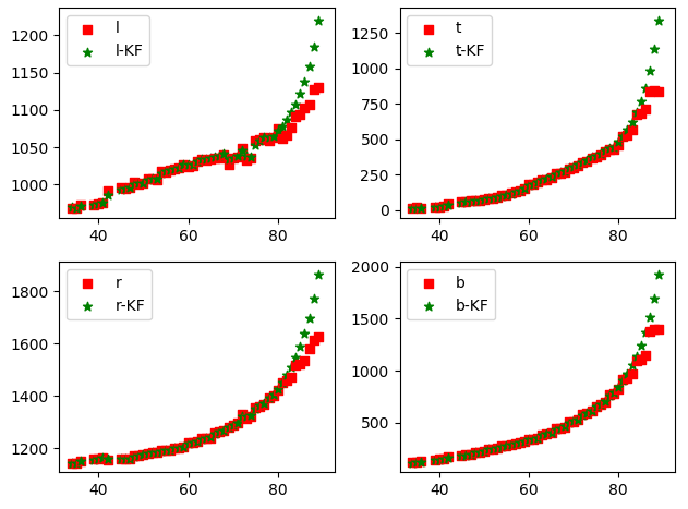
Introducing homography transformation
- State quantity: l,t,r,b, vl,vt,vr,vb
- Observation: l,t,r,b
- The observation noise variance is related to the process noise error and the bbox height. The larger the h is, the larger the error is, and it can be updated in real time
- Homography transformation matrix between calibration image and world coordinate system*
- Select mark points to build the world coordinate system
- Select the corresponding point on the image
- Calibration (bbox is not always on the plane set in the world coordinate system, so it may be a problem if it is used approximately)
- The target moves uniformly in the world coordinate system
class KalmanFilter:
    def __init__(self, homography):
        self._std_weight_pos = 1. / 10     # position
        self._std_weight_vel = 1. / 100    # speed
        self.H = np.matrix(np.zeros((4, 8)))  # Observation matrix Z_t = Hx_t + v
        for i in range(4):
            self.H[i, i] = 1
        self.F = np.matrix(np.eye(8)) # State transition matrix
        self.homography = np.reshape(homography, (3,3))

    def _img2world(self, val):
        l,t,r,b = val
        tmp = np.dot(np.linalg.inv(self.homography), np.array([[l], [t], [1]]))
        l_ = tmp[0] / tmp[2]
        t_ = tmp[1] / tmp[2]
        tmp = np.dot(np.linalg.inv(self.homography), np.array([[r], [b], [1]]))
        r_ = tmp[0] / tmp[2]
        b_ = tmp[1] / tmp[2]
        return [l_, t_, r_, b_]


    def _world2img(self, val):
        l,t,r,b = val
        tmp = np.dot(self.homography, np.array([[l], [t], [1]]))
        l_ = tmp[0] / tmp[2]
        t_ = tmp[1] / tmp[2]
        tmp = np.dot(self.homography, np.array([[r], [b], [1]]))
        r_ = tmp[0] / tmp[2]
        b_ = tmp[1] / tmp[2]
        return [l_, t_, r_, b_]

    def init(self, val):
        ltrb = self._img2world(val)
        mean_pos = np.matrix(ltrb)
        mean_vel = np.zeros_like(mean_pos) # Speed initialized to 0
        self.x_hat = np.r_[mean_pos, mean_vel] # x_k = [p, v]
        h = val[3]-val[1]
        std_pos = [
            self._std_weight_pos * h,
            self._std_weight_pos * h,
            self._std_weight_pos * h,
            self._std_weight_pos * h]
        std_vel = [
            self._std_weight_vel * h,
            self._std_weight_vel * h,
            self._std_weight_vel * h,
            self._std_weight_vel * h]
        self.P = np.diag(np.square(np.r_[std_pos, std_vel])) # State covariance matrix

    def predict(self, delt_t, val=None):
        if val is not None:
            h = val[3] - val[1]
            std_pos = [
                self._std_weight_pos * h,
                self._std_weight_pos * h,
                self._std_weight_pos * h,
                self._std_weight_pos * h]
            std_vel = [
                self._std_weight_vel * h,
                self._std_weight_vel * h,
                self._std_weight_vel * h,
                self._std_weight_vel * h]
            self.Q = np.diag(np.square(np.r_[std_pos, std_vel])) # Real time change of process noise
        for i in range(4):
            self.F[i, i+4] = delt_t
        self.x_hat_minus = self.F * self.x_hat
        self.P_minus = self.F * self.P * self.F.T + self.Q

    def update(self, val):
        l,t,r,b = val
        h = b - t
        std_pos = [
            self._std_weight_pos * h,
            self._std_weight_pos * h,
            self._std_weight_pos * h,
            self._std_weight_pos * h]
        ltrb = self._img2world(val)
        self.R = np.diag(np.square(std_pos)) # Observation noise variance
        measure = np.matrix(ltrb)
        self.K = self.P_minus * self.H.T * np.linalg.inv(self.H * self.P_minus * self.H.T + self.R)
        self.x_hat = self.x_hat_minus + self.K * (measure - self.H * self.x_hat_minus)
        self.P = self.P_minus - self.K * self.H * self.P_minus
Analysis of experimental results
-
Obviously, the uniform motion model is not suitable
-
The target vehicle is not uniformly accelerated (decelerated) in the image. The introduction of acceleration model has a nonlinear prediction effect, but it is not very good
-
Through the transformation of homography transformation, the nonlinearity is obvious and the trend is not very right. The four points adopt a homography transformation matrix, and the error is a little large
-
Detailed engineering data: Kalman filtering