House price forecast
Original question: https://www.kaggle.com/c/house-prices-advanced-regression-techniques/data?select=train.csv
reference resources: https://blog.csdn.net/qq_29153321/article/details/103967670
The house price prediction experiment analyzes 1460 house price data and the attributes of 80 houses, establishes a regression model, and then predicts the prices of 1459 new house data.
Data preprocessing
Import data
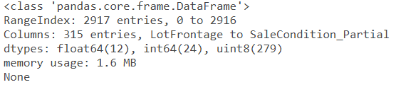
import pandas as pd
train_path = 'house-prices-advanced-regression-techniques/train.csv'
train = pd.read_csv(train_path)
test_path = 'house-prices-advanced-regression-techniques/test.csv'
test = pd.read_csv(test_path)
print(train.head())
print(train.info())
Out: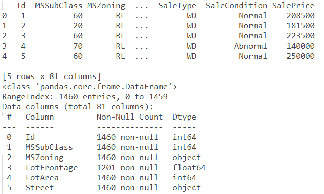
Weed out useless columns
It is easy to get from the characteristics and purpose: 'Id' belongs to the sequence and does not help predict house prices. Delete it
train.drop('Id', axis = 1, inplace = True)
test.drop('Id', axis = 1, inplace = True)
print(train.head())
Out: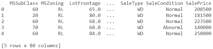
(pandas.DataFrame).drop()
Parameter Description:
First parameter: Specifies the index to be deleted
Axis: processed by row (axis = 0) or column (axis = 1). The default value is 0
inplace: whether to directly operate the original data. The default value is False
Detect outliers
According to the problem prediction analysis, the aboveground living area will be a major factor affecting the house price, so the visual display will check whether there are abnormal values
import matplotlib.pyplot as plt
train.plot(kind = 'scatter', x = 'GrLivArea', y = 'SalePrice', alpha = 0.2, figsize = (10, 8))
plt.ylabel('SalePrice', fontsize = 13)
plt.xlabel('GrLivArea', fontsize = 13)
plt.grid()
plt.show()
Out: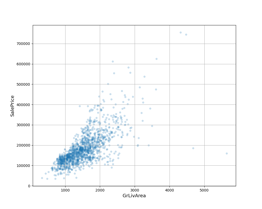
It can be seen that there are two outliers in the lower right corner (large area but low price). Delete the outliers directly
train = train.drop(train[(train['GrLivArea']>4000) & (train['SalePrice']<300000)].index)
This statement is divided into several layers:
train[(train ['GrLivArea '] > 4000) & (train ['SalePrice'] < 300000)]: data division, filter out qualified data, format: df [(condition)]
. index: returns the index value
. drop(): deletes the specified data according to the index
Modified label distribution
For linear regression models, it is an important step to check whether the label distribution conforms to the normal distribution and correct it
Because when the variable follows the normal distribution, the probability of predicting the variable and finding it within a certain range will become very simple
import seaborn as sns
sns.distplot(train['SalePrice'])
plt.ylabel('Frequency')
plt.title('SalePrice distribution')
plt.show()
Out: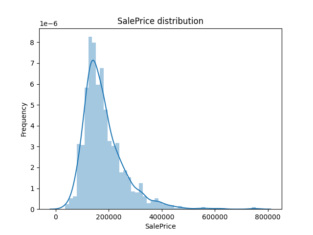
It can be seen that the price distribution is inclined to the left. If you want to correct it, you need to expand the low price area and compress the high price area. log(1+x) is used to convert and correct the SalePrice. Of course, in the subsequent application of the model, you should pay attention to the label transformation
import numpy as np
train['SalePrice'] = np.log1p(train['SalePrice'])
sns.distplot(train['SalePrice'])
plt.ylabel('Frequency')
plt.title('SalePrice distribution')
plt.show()
Out: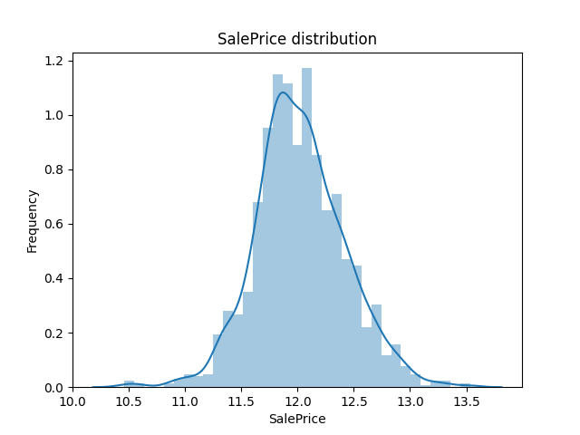
Merge datasets
The training set and test set are combined for data preprocessing without repeated work
len_train = len(train)
len_test = len(test)
y_train = train['SalePrice']
all_data = pd.concat((train, test), axis = 0).reset_index(drop = True)
all_data.drop(['SalePrice'], axis = 1, inplace = True)
df.concat((A, B), axis = 0).reset_index(drop = True) means to merge up and down matrices A and B (axis = 0), and delete the original row indexes of the two matrices
Missing value processing
First, make statistics on which fields have missing data and what are the missing rates
def get_missing_data_summary(my_dataframe):
    all_data_na = (my_dataframe.isnull().sum() / len(my_dataframe)) * 100
	all_data_na = all_data_na.drop(all_data_na[all_data_na == 0].index).sort_values(ascending=False)
    missing_data = pd.DataFrame({'Missing Ratio (%)' :all_data_na})
    return missing_data
missing_data = pd.DataFrame({'Missing Ratio (%)' :all_data_na})
print(missing_data)
Out: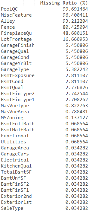
It can be seen that there are many features with missing data, which need to be processed according to the specific business significance of the features
Class I: the missing value also belongs to one of the characteristic values (for example, PoolQC is the information related to the swimming pool, and the missing value indicates that there is no swimming pool)
C1 = ['PoolQC', 'MiscFeature', 'Alley', 'Fence', 'FireplaceQu', 'GarageType', 'GarageFinish', 'GarageQual', 'GarageCond','BsmtQual', 'BsmtCond', 'BsmtExposure', 'BsmtFinType1', 'BsmtFinType2', 'MasVnrType']
for col in C1:
    all_data[col].fillna('None', inplace = True)
Type II: numerical type characteristics, which should be assigned as 0 according to the analysis (for example, if there is no garage, the corresponding relevant information, such as garage area, can be directly assigned as 0)
C2 = ['GarageYrBlt', 'GarageArea', 'GarageCars', 'BsmtFinSF1', 'BsmtFinSF2', 'BsmtUnfSF', 'TotalBsmtSF', 'BsmtFullBath','BsmtHalfBath', 'MasVnrArea']
for col in C2:
    all_data[col].fillna(0, inplace = True)
The third category: most of the deficiencies that do not belong to the first two categories are illogical, and their modes are used to fill them
C3 = ['MSZoning', "Functional", 'Electrical', 'KitchenQual', 'Exterior1st', 'Exterior2nd', 'SaleType', 'MSSubClass']
for col in C3:
    all_data[col].fillna(all_data[col].mode()[0], inplace = True)
Category 4: a special feature: 'Utilities'. All non missing values are the same value, which is meaningless. They are simply deleted
all_data.drop('Utilities', axis = 1, inplace = True)
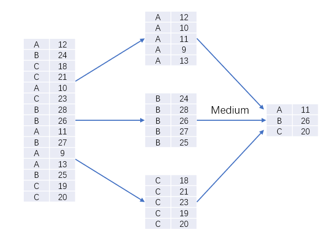
Category 5: a special feature: 'LotFrontage', which is "linear Street feet connected to the property", while another feature, 'Neighborhood', indicates "the geographical area where the house is located". Obviously, the distance between the house and the property in the same area is almost the same, so the missing value can be replaced by the median of the 'LotFrontage' value in the same area
all_data["LotFrontage"] = all_data.groupby("Neighborhood")["LotFrontage"].transform(lambda x: x.fillna(x.median()))
df.groupby('A ') [' B '). transform(lambda x: c): divide the data into several categories according to the value of column A (several values in column A are divided into several categories), and then replace the value of B in each category with c
This statement means: classify the samples according to the feature "Neighborhood", name the "LotFrontage" value of each class as X, and replace the x value of this class with the median of X of this class
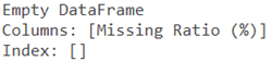
Review the characteristics of missing data again
missing_data = pd.DataFrame({'Missing Ratio (%)' :all_data_na})
print(missing_data)
Out:
Handling special attributes
all_data['MSSubClass'] = all_data['MSSubClass'].apply(str)
Although MSSubClass is a numeric type, it actually uses numeric values to distinguish house types. The values themselves are not comparable in size, so they are converted to character types for subsequent encoding processing
Combination feature
Generate a new field: total house area
According to business knowledge, this feature may be useful for house price prediction
all_data['TotalSF'] = all_data['TotalBsmtSF'] + all_data['1stFlrSF'] + all_data['2ndFlrSF']
Processing category data as dummy variables
all_data = pd.get_dummies(all_data, drop_first = True)
print(all_data.info())
Out:
The characteristics of non numerical classes in the matrix are treated as dummy variables and inserted back into the original matrix, and the matrix will be expanded accordingly
Split dataset
X_train = all_data[:len_train].values
X_test = all_data[len_train:].values
Re split the data set into training set and test set
Feature scaling
from sklearn.preprocessing import StandardScaler
sc_X = StandardScaler()
X_train = sc_X.fit_transform(X_train)
X_test = sc_X.transform(X_test)
y_train = np.array(y_train).reshape(-1, 1)
Feature scaling is often used as the last step of data preprocessing. It is suggested that feature scaling is needed before building a model
Select model
Establish regression model
#Lasso
from sklearn.linear_model import Lasso
lasso = Lasso(alpha = 0.0005, random_state = 1)

#Elastic Net Regression
from sklearn.linear_model import ElasticNet
enet = ElasticNet(alpha = 0.0005, l1_ratio = 0.9, random_state = 3)

#Kernel Ridge Regression
from sklearn.kernel_ridge import KernelRidge
krr = KernelRidge(alpha = 0.6, kernel = 'polynomial', degree = 2, coef0 = 2.5)

#Gradient Boosting Regression
from sklearn.ensemble import GradientBoostingRegressor
gboost = GradientBoostingRegressor(n_estimators = 3000, learning_rate = 0.05, max_depth = 4, max_features = 'sqrt',
                                   min_samples_leaf = 15, min_samples_split = 10, loss = 'huber', random_state = 5)

#random forest
from sklearn.ensemble import RandomForestRegressor
rf = RandomForestRegressor(n_estimators = 500, random_state = 0)

#XGBoost
import xgboost as xgb
xgb = xgb.XGBRegressor(colsample_bytree = 0.4, gamma = 0.05, learning_rate = 0.05, max_depth = 3, min_child_weight = 2,
                       n_estimators = 2200, reg_alpha = 0.5, reg_lambda = 0.9, subsample = 0.5,silent = 1, random_state = 7,
                       nthread = -1)

#LightGBM
import lightgbm as lgb
lgb = lgb.LGBMRegressor(objective = 'regression', num_leaves = 5, learning_rate = 0.05, n_estimators = 720,
                        max_bin = 55, bagging_fraction = 0.8, bagging_freq = 5, feature_fraction = 0.25,
                        feature_fraction_seed = 9, bagging_seed = 9, min_child_samples = 6, min_child_weight = 11)
Model performance evaluation and selection
k-fold cross validation is generally used in the industry to evaluate the model performance. Here, k=10. There are two evaluation indicators, one is r^2 (r squared), which is used to judge the model performance; the other is mse (mean squared error), which is used to observe the variance. In order to speed up the execution speed, n_jobs = 2 means using two CPUs (two core CPUs) verbose = 1 indicates that information is continuously printed out during execution to help judge how much is executed
#K-fold
from sklearn.model_selection import cross_val_score
def evaluation_model(model):
	rmse = np.sqrt(-cross_val_score(estimator = model, X = X_train, y = y_train, scoring = 'neg_mean_squared_error',
                                    cv = 10, n_jobs = 2, verbose = 1))
	r2_score = cross_val_score(estimator = model, X = X_train, y = y_train, scoring = 'r2', cv = 10, n_jobs = 2, verbose = 1)
	return (r2_score, rmse)
#running
lasso_r2, lasso_rmse = evaluation_model(lasso)
enet_r2, enet_rmse = evaluation_model(enet)
krr_r2, krr_rmse = evaluation_model(krr)
gboost_r2, gboost_rmse = evaluation_model(gboost)
rf_r2, rf_rmse = evaluation_model(rf)
xgb_r2, xgb_rmse = evaluation_model(xgb)
lgb_r2, lgb_rmse = evaluation_model(lgb)
Out: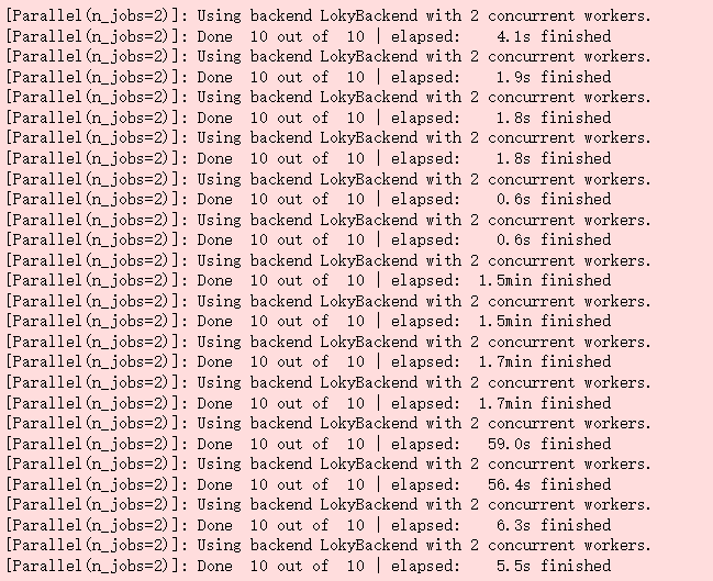
#print result function
def print_result(r2_score, rmse, model_name):
	print('%s evaluation:r2 = %.4f(std = %.4f), rmse = %.4f(std = %.4f)'
          %(model_name, r2_score.mean(), r2_score.std(), rmse.mean(), rmse.std()))
	return 0
#print result
print_result(lasso_r2, lasso_rmse, 'Lasso')
print_result(enet_r2, enet_rmse, 'Elastic Net')
print_result(krr_r2, krr_rmse, 'Kernel Redge')
print_result(gboost_r2, gboost_rmse, 'Gradient Boost')
print_result(rf_r2, rf_rmse, 'Random Forest')
print_result(xgb_r2, xgb_rmse, 'XG Boost')
print_result(lgb_r2, lgb_rmse, 'Lightgbm')
Out:
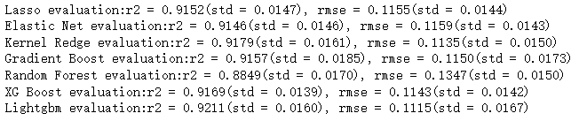
We found that Linghtgbm has the best performance (R2 > 0.9, and mse and std are small), so we chose Lightgbm model for further optimization
Model performance optimization
Debug the super parameters of the model and optimize the data of the project to obtain better regression data.
LightGBM parameter adjustment method:
- Select a higher learning rate to accelerate the convergence speed and improve the parameter adjustment efficiency
- Adjusting the basic parameters of decision tree
- Regularization parameter tuning
- Reduce learning rate and improve accuracy
Get the number of iterations under the current learning rate
Using the cv function of LightGBM, the initial values of model parameters are set simply according to the problem
LightGBM parameters: https://lightgbm.readthedocs.io/en/latest/pythonapi/lightgbm.LGBMRegressor.html#lightgbm.LGBMRegressor
How to use lightgbm.cv function: https://blog.csdn.net/weixin_44414593/article/details/108727307
import lightgbm as lgb

params = {
    'boosting_type':'gbdt',
    'objective':'regression',
    'n_jobs':-1
    'learning_rate':0.1,
    'num_leaves':15,
    'max_depth':5,
    'subsample':0.8,
    'colsample_bytree':0.8
}
data_train = lgb.Dataset(X_train, y_train, silent = True)
cv_results = lgb.cv(params, data_train, nfold = 5, metrics = 'rmse', num_boost_round = 1000, early_stopping_rounds = 50,
                    verbose_eval = 50, stratified = False, seed = 0)
print('best n_estimators:', len(cv_results['rmse-mean']))
print('best cv score:', cv_results['rmse-mean'][-1])
Out:
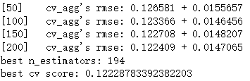
It can be seen that when the learning rate is 0.1, the optimal number of iterations is 194, so we next use learning_rate = 0.1, num_boost_round = 194
Basic commissioning parameters
Use GridSearchCV() in sklearn to perform grid search, coarse adjustment first and then fine adjustment
GridSearchCV() reference: https://blog.csdn.net/weixin_41988628/article/details/83098130?ops_request_misc=%257B%2522request%255Fid%2522%253A%2522163444549716780269819093%2522%252C%2522scm%2522%253A%252220140713.130102334...%2522%257D&request_id=163444549716780269819093&biz_id=0&utm_medium=distribute.pc_search_result.none-task-blog-2alltop_positive~default-1-83098130.first_rank_v2_pc_rank_v29&utm_term=GridSearchCV&spm=1018.2226.3001.4187
Simply set the initial value first
from sklearn.model_selection import GridSearchCV

model_lgb = lgb.LGBMRegressor(object = 'regression', num_leaves = 15, learning_rate = 0.1, n_estimators = 194, max_depth = 5,
                              metric = 'rmse', bagging_fraction = 0.8, feature_fraction = 0.8)
Important parameters to improve accuracy
max_depth: the depth of the tree. If the depth is too large, it may be too fitted
Num_leaves: the complexity of the tree. It is required that num_leaves < 2 ^ (max_depth), otherwise it will be over fitted
params_test1 = {'max_depth':range(3, 10, 2), 'num_leaves':range(5, 125, 20)}
gsearch1 = GridSearchCV(estimator = model_lgb, param_grid = params_test1, scoring = 'neg_mean_squared_error', cv = 5,
                        verbose = 1, n_jobs = -1)
gsearch1.fit(X_train, y_train)
gsearch1.best_params_, gsearch1.best_score_
Out:

Here, the lower the mean square error (rmse) used in the metric strategy, the better. sklearn provides neg_mean_squared_error and returns the rmse of metric. Similarly, the closer it is to 0, the better
The range is reduced several times according to the results, and finally the best super parameters are obtained:
params_test1 = {'max_depth':range(2, 5, 1), 'num_leaves':range(5, 10, 1)}
gsearch1 = GridSearchCV(estimator = model_lgb, param_grid = params_test1, scoring = 'neg_mean_squared_error', cv = 5,
                        verbose = 1, n_jobs = -1)
gsearch1.fit(X_train, y_train)
gsearch1.best_params_, gsearch1.best_score_
Out:

Reduce the important parameters of over fitting
min_child_samples: also known as min_data_in_leaf, the minimum number of data on a leaf. It can be used to process over fitting
min_child_weight: also known as min_sum_hessian_in_leaf, the minimum Hessian sum on a leaf can be used to deal with over fitting
params_test2 = {'min_child_samples':range(0, 40, 10), 'min_child_weight':range(0, 20, 2)}
model_lgb = lgb.LGBMRegressor(objective = 'regression', num_leaves = 6, learning_rate = 0.1, n_estimators = 194, max_depth = 3,
                              metric = 'rmse', bagging_fraction = 0.8, feature_fraction = 0.8)
gsearch2 = GridSearchCV(estimator = model_lgb, param_grid = params_test2, scoring = 'neg_mean_squared_error', cv = 5,
                        verbose = 1, n_jobs = -1)
gsearch2.fit(X_train, y_train)
gsearch2.best_params_, gsearch2.best_score_
Out:

Further narrow the scope:
params_test2 = {'min_child_samples':range(0, 10, 1), 'min_child_weight':range(5, 10, 1)}
model_lgb = lgb.LGBMRegressor(objective = 'regression', num_leaves = 6, learning_rate = 0.1, n_estimators = 194, max_depth = 3,
                              metric = 'rmse', bagging_fraction = 0.8, feature_fraction = 0.8)
gsearch2 = GridSearchCV(estimator = model_lgb, param_grid = params_test2, scoring = 'neg_mean_squared_error', cv = 5,
                        verbose = 1, n_jobs = -1)
gsearch2.fit(X_train, y_train)
gsearch2.best_params_, gsearch2.best_score_
Out:

Reduce the other two parameters of over fitting
feature_fraction: also known as colsample_bytree, it is used for sub sampling of features to prevent over fitting and improve training speed
bagging_fraction: also known as subsample, it is the sample sampling proportion of the training instance, which can make bagging run faster and reduce fitting.
bagging_freq: also called subsample_freq, 0 by default, indicates the frequency of bagging. 0 means that bagging is not used, and K means that bagging is performed every k rounds of iteration.
params_test3 = {
    'feature_fraction':[0.1, 0.3, 0.5, 0.7, 0.9, 1],
    'bagging_fraction':[0.1, 0.3, 0.5, 0.7, 0.9, 1]
    'bagging_freq':range(0, 10)
}
model_lgb = lgb.LGBMRegressor(objective = 'regression', num_leaves = 6, learning_rate = 0.1, n_estimators = 194, max_depth = 3,
                              metric = 'rmse', bagging_fraction = 0.8, feature_fraction = 0.8, min_child_samples = 6,
                              min_child_weight = 7)
gsearch3 = GridSearchCV(estimator = model_lgb, param_grid = params_test3, scoring = 'neg_mean_squared_error', cv = 5,
                        verbose = 1, n_jobs = -1)
gsearch3.fit(X_train, y_train)
gsearch3.best_params_, gsearch3.best_score_
Out:

params_test3 = {
    'feature_fraction':[0.25, 0.3, 0.35, 0.4, 0.45],
    'bagging_fraction':[0.86, 0.88, 0.9, 0.92, 0.94],
    'bagging_freq':[1, 2, 3, 4]
}
model_lgb = lgb.LGBMRegressor(objective = 'regression', num_leaves = 6, learning_rate = 0.1, n_estimators = 194, max_depth = 3,
                              metric = 'rmse', bagging_fraction = 0.8, feature_fraction = 0.8, min_child_samples = 6,
                              min_child_weight = 7)
gsearch3 = GridSearchCV(estimator = model_lgb, param_grid = params_test3, scoring = 'neg_mean_squared_error', cv = 5,
                        verbose = 1, n_jobs = -1)
gsearch3.fit(X_train, y_train)
gsearch3.best_params_, gsearch3.best_score_
Out:

Regularization parameters
lambda_l1: L1 regularization coefficient
lambda_l2: L2 regularization coefficient
params_test4 = {
    'lambda_l1': [0, 0.001, 0.01, 0.03, 0.08, 0.3, 0.5],
    'lambda_l2': [0, 0.001, 0.01, 0.03, 0.08, 0.3, 0.5]
}
model_lgb = lgb.LGBMRegressor(objective = 'regression', num_leaves = 6, learning_rate = 0.1, n_estimators = 194, max_depth = 3,
                              metric = 'rmse', bagging_fraction = 0.01, feature_fraction = 0.41, min_child_samples = 6,
                              min_child_weight = 7)
gsearch4 = GridSearchCV(estimator = model_lgb, param_grid = params_test4, scoring = 'neg_mean_squared_error', cv = 5,
                        verbose = 1, n_jobs = -1)
gsearch4.fit(X_train, y_train)
gsearch4.best_params_, gsearch4.best_score_
Out:

Reduce learning rate
Higher learning rate was used before because it can make convergence faster, but accuracy is bound to be sacrificed. A lower learning rate and more decision trees are used here n_estimators to train data, trying to get a better model
params = {
    'boosting_type':'gbdt',
    'objective':'regression',
    'n_jobs':-1,
    'learning_rate':0.005,
    'num_leaves':6,
    'max_depth':3,
    'bagging_fraction':0.92,
    'bagging_freq':2,
    'colsample_bytree':0.4,
    'min_child_samples':6,
    'min_child_weight':7,
    'lambda_l1':0,
    'lambda_l2':0.01
}
data_train = lgb.Dataset(X_train, y_train, silent = True)
cv_results = lgb.cv(params, data_train, nfold = 5,  metrics = 'rmse', num_boost_round = 10000, early_stopping_rounds = 50,
                    verbose_eval = 100, stratified = False, seed = 0, show_stdv = True)
print('best n_estimators:', len(cv_results['rmse-mean']))
print('best cv score:', cv_results['rmse-mean'][-1])
Out:
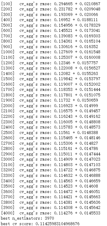
The optimal number of iterations is 3970
Establish the best model for prediction
According to the optimization, we get the best model
import lightgbm as lgb

regressor = lgb.LGBMRegressor(
    boosting_type = 'gbdt',
    objective = 'regression',
    n_jobs = -1,
    n_estimators = 3970,
    learning_rate = 0.005,
    num_leaves = 6,
    max_depth = 3,
    bagging_fraction = 0.92,
    bagging_freq = 2,
    colsample_bytree = 0.4,
    min_child_samples = 6,
    min_child_weight = 7,
    lambda_l2 = 0.01
)
Training model
regressor.fit(X_train, y_train)
y_pred = regressor.predict(X_test)
y_pred = np.expm1(y_pred)#The label distribution is corrected during data preprocessing, which needs to be corrected
test_set = pd.DataFrame(np.arange(0, X_test.shape[0]).reshape(-1, 1))
test_set['SalePrice'] = y_pred
test_set.to_csv('test_set.csv')
effect

The effect can only be said reluctantly...
This article is my study notes, focusing on learning the whole regression project process. Leaders are welcome to put forward suggestions in the comment area.