1. K-Nearest Neighbor Algorithms

The configuration is as follows

• System Ubuntu Kylin
• IDE  Pycharm Community
• Language Python 3
  

2. Module Installation

After installing Python 3 and IDE, we need to first install the relevant modules (i.e. function libraries) so that we can complete the next study.

1. pip3 installation

sudo apt-get install python3-pip

Function: Used to provide the library required by Python 3.

2. Numpy installation

 pip3 install numpy

Functions: Function libraries used to provide matrix operations

3. Matplotlib installation

 pip3 install pillow

Function: Install python image processing library

sudo apt-get install python3-tk

Function: Install the GUI interface tkinter Library

 sudo apt-get install libfreetype6-dev libxft-dev
 sudo pip3 install matplotlib

Function: Install matplotlib drawing library

4. Use of Matplotlib

import matplotlib
matplotlib.use('Qt5Agg')

Function: In actual use, you need to add statements to display them.

3. Overview of k-Nearest Neighbor Algorithms

k-NN is a type of instance-based learning, or lazy learning, where the function is only approximated locally and all computation is deferred until classification. The k-NN algorithm is among the simplest of all machine learning algorithms. - [ Wikipedia ]

Simply put, k-nearest neighbor algorithm classifies by measuring the distance between different eigenvalues.

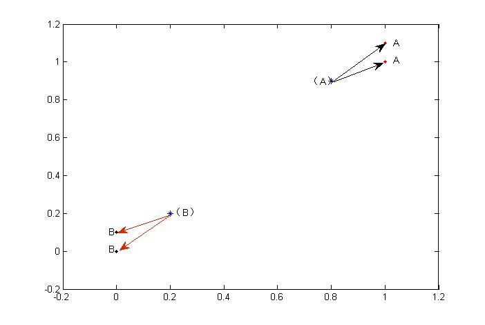
As shown in the figure, in the case of known classification labels (red A and black B points in the figure), classification is carried out by calculating the distance between the points to be classified (blue*) and the known labels.

k-nearest neighbor

Advantage:	High accuracy, insensitive to outliers, no data input assumptions
Disadvantages:	High computational complexity and high spatial complexity
Use data range:	NUMERICAL AND NORMAL TYPES

4. Specific examples

Here are two examples to illustrate how to use python to implement kNN algorithm.

1. Matching effect of dating website

My friend Helen has been using online dating sites to find suitable dates. Although dating websites recommend different people, she doesn't like everyone. After summing up, she found that she had met three types of people:

• A disliked person
• Charming people
• Charming people

Like many girls, Helen wants to date attractive people from Monday to Friday and spend the weekend with attractive people. Helen hopes to have such a classification software to help her better classify matched objects into exact categories. In addition, Helen has collected some data information that has not been recorded on dating websites, which she believes is more helpful in categorizing matches.

Helen stores these data in a text file, with each sample data occupying one row, totaling 1,000 rows. Helen's sample data contains the following three characteristics:

• Frequent Flight Mileage Obtained Annually
• Percentage of time spent playing video games
• Ice-cream litres consumed per week

First, we need to complete the format processing program, which is as follows:

# ----------------------------------------------------------------------------------------------------------------------------------------
def file2matrix(filename):
    fr = open(filename)
    # Read text
    arrayOLines = fr.readlines()
    # Calculate the number of lines of text
    numberOfLines = len(arrayOLines)
    # Construct a zero matrix with dimension: rows*3
    returnMat = zeros((numberOfLines, 3))
    # Construct a label vector to return label values
    classLabelVector = []
    # Construct an index to select rows of a matrix
    index = 0
    for line in arrayOLines:
        # Remove carriage return
        line = line.strip()
        # Segmentation of strings usingt as a file delimiter
        listFromLine = line.split('\t')
        # Filling Matrix
        returnMat[index,:] = listFromLine[0:3]
        # Add the last column of the list to the label
        classLabelVector.append(int(listFromLine[-1]))
        # Processing the next line
        index += 1
return returnMat, classLabelVector

Next, we use Matplotlib to make scatter plots of the original data, so that we can observe the characteristics of the data very well.

# Import data - -------------------------------------------------------------------------------------
datingDataMat, datingLabels = file2matrix('datingTestSet2.txt')
print(datingDataMat)
print(datingLabels[0:20])

# Analytical data - -----------------------------------------------------------------------------------------------------------------------------
# Creating scatter plots using Matplotlib

# matplotlib installation:
# 1. sudo apt-get install libfreetype6-dev libxft-dev
# 2. sudo pip3 install matplotlib
import matplotlib
# Show scatter plot
matplotlib.use('Qt5Agg')
# matplotlib.matplotlib_fname()
import matplotlib.pyplot as plt

fig = plt.figure()
# Setting Picture Display Location Information
ax = fig.add_subplot(111)
# Setting Picture Scattering Information
ax.scatter(datingDataMat[:,1], datingDataMat[:,2])
plt.show()

# Calling scatter function to personalize marking points on scatter graph
fig1 = plt.figure()
ax = fig1.add_subplot(111)
ax.scatter(datingDataMat[:,1], datingDataMat[:,2],
           15.0*array(datingLabels), 15.0*array(datingLabels))
plt.show()

Considering the magnitude differences among the three types of data, such as frequent flyer mileage is much larger than the percentage of time consumed by video games, we need to normalize the data:

# Preparing data - -----------------------------------------------------------------------------------------------------------------------
# Data normalization
def autoNorm(dataSet):
    # Column Minimum (Minimum values can be selected from columns using min(0); Minimum values can be selected from rows using min(1)
    minVals = dataSet.min(0)
    # Column maximum
    maxVals = dataSet.max(0)
    # Section
    ranges = maxVals - minVals
    # Constructing Zero Vector
    normDataSet = zeros(shape(dataSet))
    # Determine the number of rows
    m = dataSet.shape[0]
    # Determinant subtraction (note: using determinant instead of cycle can increase speed)
    normDataSet = dataSet - tile(minVals, (m,1))
    # Determinant division (the same advantages)
    normDataSet = normDataSet/tile(ranges, (m,1))
return normDataSet, ranges, minVals

Finally, we have to complete the preparation of classifiers:

# inX: input vectors for classification; dataSet: training sample set for input; labels: label vectors; k: number of nearest neighbors for selection
def classify0(inX, dataSet, labels, k):
    # Read the length of the first dimension of the matrix at http://www.cnblogs.com/zuizui1204/p/6511050.html
    dataSetSize = dataSet.shape[0]
    # tile: Repeat the dimension and expand it. Reference website: http://blog.csdn.net/wy250229163/article/details/52453201
    # diffMat: Represents the distance between the input vector and the training sample set
    diffMat = tile(inX, (dataSetSize, 1)) - dataSet
    # Calculate squares: a^2,b^2 (d=sqrt(a^2+b^2))
    sqDiffMat = diffMat**2
    # Add each row of elements of the matrix: a^2+b^2. If axis=0, it is a general summation.
    sqDistances = sqDiffMat.sum(axis = 1)
    # Calculate the radical of distance
    distances = sqDistances**0.5
    # Sort by distance and return the index
    sortedDistIndices = distances.argsort()
    classCount = {}
    # Choosing the k Points with the Minimum Distance
    for i in range(k):
        # Get the label value
        voteIlabel = labels[sortedDistIndices[i]]
        # Calculate the number of label appearances
        classCount[voteIlabel] = classCount.get(voteIlabel, 0) + 1
    # In descending order according to the number of label appearances. Note: Use items instead of iteritems in Python 3
    sortedClassCount = sorted(classCount.items(),
                              key = operator.itemgetter(1), reverse = True)
    return sortedClassCount[0][0]

Next, we can test the error rate of our classification and see if Helen can get what she wants.

# Test algorithm
def datingClassTest():
    # The code here is explained before
    hoRatio = 0.10
    datingDataMat, datingLabels = file2matrix('datingTestSet2.txt')
    normMat, ranges, minVals = autoNorm(datingDataMat)
    m = normMat.shape[0]
    # The test data is 10%.
    numTestVecs = int(m*hoRatio)
    # Initialization error rate
    errorCount = 0.0
    # Judge the classification of each test data
    for i in range(numTestVecs):
        # Using classifier training, the training data is 90%.
        classifierResult = classify0(normMat[i,:], normMat[numTestVecs:m,:],
                                     datingLabels[numTestVecs:m], 3)
        print("the classifier came back with: %d, the real answer is: %d"
              % (classifierResult, datingLabels[i]))
        if (classifierResult != datingLabels[i]):
            errorCount += 1.0
    print("the total error rate is: %f" % (errorCount/float(numTestVecs)))

# Output results
datingClassTest()

2. Handwritten Number Recognition System

In the handwritten recognition system, we train classifiers to determine handwritten digits, where each handwritten digit can be represented by a binary image matrix as shown below:

Next, handwritten digit recognition can be completed by image conversion and classifier decision. For the specific implementation code of this section, please refer to: Handwritten Number Recognition System

5. References

Books: Machine Learning Practice

Source code: Git of SchrodengerY