this is the second article on the introduction to PyTorch. It will be continuously updated as a series of PyTorch articles.
this paper will introduce how to use PyTorch to build a simple MLP (Multi-layer Perceptron) model to realize two classification and multi classification tasks.
Data set introduction
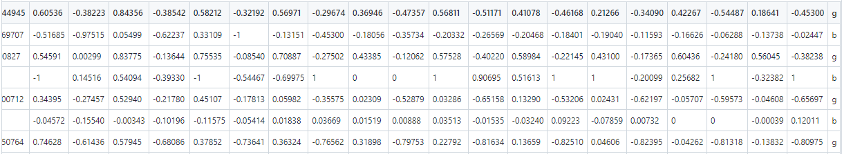
the second classification data set is ionosphere.csv (ionosphere data set), which is UCI machine learning dataset Classical binary dataset in. It has 351 observations, 34 independent variables and 1 dependent variable (category). The category values are g(good) and b(bad). In the ionosphere.csv file, there are 351 lines. The first 34 columns are used as arguments (input X) and the last column is used as category value (output y).
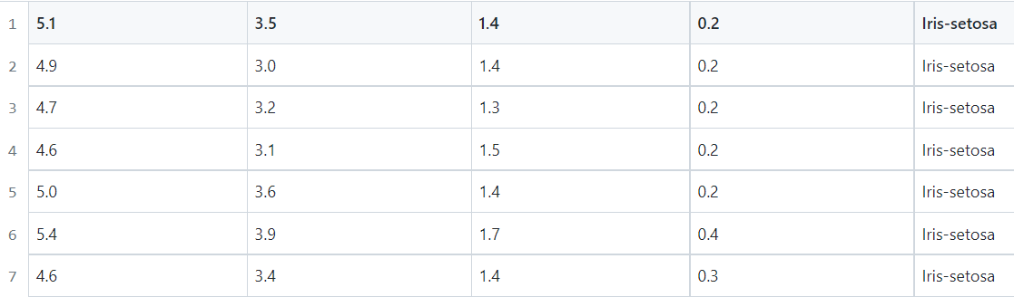
The multi classification dataset is iris.csv (iris dataset), which is UCI machine learning dataset Classical multi classification dataset in. It has a total of 150 observations, 4 independent variables (sepal length, sepal width, petal length, petal width) and 1 dependent variable (category). The category values are iris setosa, iris versicolor and iris virgin. In the iris.csv file, there are 150 lines. The first four columns are used as arguments (input X) and the last column is used as category value (output y). The first few lines of data are shown in the figure below:
Classification model process
the basic process of using PyTorch to build a neural network model to solve the classification problem is as follows:
Among them, loading data set and dividing data set are the data processing part, building model and selecting loss function and optimizer are the part of creating model. The goal of model training is to select appropriate optimizer and training step to make the value of loss function very small. Model prediction is the prediction on model test set or new data.
Binary classification model
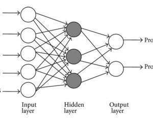
use PyTorch to build an MLP model to realize the secondary classification task. The model results are as follows:
The Python code for implementing the MLP model is as follows:
# -*- coding: utf-8 -*-
# pytorch mlp for binary classification
from numpy import vstack
from pandas import read_csv
from sklearn.preprocessing import LabelEncoder
from sklearn.metrics import accuracy_score
from torch import Tensor
from torch.optim import SGD
from torch.utils.data import Dataset, DataLoader, random_split
from torch.nn import Linear, ReLU, Sigmoid, Module, BCELoss
from torch.nn.init import kaiming_uniform_, xavier_uniform_


# dataset definition
class CSVDataset(Dataset):
    # load the dataset
    def __init__(self, path):
        # load the csv file as a dataframe
        df = read_csv(path, header=None)
        # store the inputs and outputs
        self.X = df.values[:, :-1]
        self.y = df.values[:, -1]
        # ensure input data is floats
        self.X = self.X.astype('float32')
        # label encode target and ensure the values are floats
        self.y = LabelEncoder().fit_transform(self.y)
        self.y = self.y.astype('float32')
        self.y = self.y.reshape((len(self.y), 1))

    # number of rows in the dataset
    def __len__(self):
        return len(self.X)

    # get a row at an index
    def __getitem__(self, idx):
        return [self.X[idx], self.y[idx]]

    # get indexes for train and test rows
    def get_splits(self, n_test=0.3):
        # determine sizes
        test_size = round(n_test * len(self.X))
        train_size = len(self.X) - test_size
        # calculate the split
        return random_split(self, [train_size, test_size])


# model definition
class MLP(Module):
    # define model elements
    def __init__(self, n_inputs):
        super(MLP, self).__init__()
        # input to first hidden layer
        self.hidden1 = Linear(n_inputs, 10)
        kaiming_uniform_(self.hidden1.weight, nonlinearity='relu')
        self.act1 = ReLU()
        # second hidden layer
        self.hidden2 = Linear(10, 8)
        kaiming_uniform_(self.hidden2.weight, nonlinearity='relu')
        self.act2 = ReLU()
        # third hidden layer and output
        self.hidden3 = Linear(8, 1)
        xavier_uniform_(self.hidden3.weight)
        self.act3 = Sigmoid()

    # forward propagate input
    def forward(self, X):
        # input to first hidden layer
        X = self.hidden1(X)
        X = self.act1(X)
        # second hidden layer
        X = self.hidden2(X)
        X = self.act2(X)
        # third hidden layer and output
        X = self.hidden3(X)
        X = self.act3(X)
        return X


# prepare the dataset
def prepare_data(path):
    # load the dataset
    dataset = CSVDataset(path)
    # calculate split
    train, test = dataset.get_splits()
    # prepare data loaders
    train_dl = DataLoader(train, batch_size=32, shuffle=True)
    test_dl = DataLoader(test, batch_size=1024, shuffle=False)
    return train_dl, test_dl


# train the model
def train_model(train_dl, model):
    # define the optimization
    criterion = BCELoss()
    optimizer = SGD(model.parameters(), lr=0.01, momentum=0.9)
    # enumerate epochs
    for epoch in range(100):
        # enumerate mini batches
        for i, (inputs, targets) in enumerate(train_dl):
            # clear the gradients
            optimizer.zero_grad()
            # compute the model output
            yhat = model(inputs)
            # calculate loss
            loss = criterion(yhat, targets)
            # credit assignment
            loss.backward()
            print("epoch: {}, batch: {}, loss: {}".format(epoch, i, loss.data))
            # update model weights
            optimizer.step()


# evaluate the model
def evaluate_model(test_dl, model):
    predictions, actuals = [], []
    for i, (inputs, targets) in enumerate(test_dl):
        # evaluate the model on the test set
        yhat = model(inputs)
        # retrieve numpy array
        yhat = yhat.detach().numpy()
        actual = targets.numpy()
        actual = actual.reshape((len(actual), 1))
        # round to class values
        yhat = yhat.round()
        # store
        predictions.append(yhat)
        actuals.append(actual)
    predictions, actuals = vstack(predictions), vstack(actuals)
    # calculate accuracy
    acc = accuracy_score(actuals, predictions)
    return acc


# make a class prediction for one row of data
def predict(row, model):
    # convert row to data
    row = Tensor([row])
    # make prediction
    yhat = model(row)
    # retrieve numpy array
    yhat = yhat.detach().numpy()
    return yhat


# prepare the data
path = './data/ionosphere.csv'
train_dl, test_dl = prepare_data(path)
print(len(train_dl.dataset), len(test_dl.dataset))
# define the network
model = MLP(34)
print(model)
# train the model
train_model(train_dl, model)
# evaluate the model
acc = evaluate_model(test_dl, model)
print('Accuracy: %.3f' % acc)
# make a single prediction (expect class=1)
row = [1, 0, 0.99539, -0.05889, 0.85243, 0.02306, 0.83398, -0.37708, 1, 0.03760, 0.85243, -0.17755, 0.59755, -0.44945,
       0.60536, -0.38223, 0.84356, -0.38542, 0.58212, -0.32192, 0.56971, -0.29674, 0.36946, -0.47357, 0.56811, -0.51171,
       0.41078, -0.46168, 0.21266, -0.34090, 0.42267, -0.54487, 0.18641, -0.45300]
yhat = predict(row, model)
print('Predicted: %.3f (class=%d)' % (yhat, yhat.round()))
In the above code, CSVDataset class is the loading class of csv dataset, which is processed into the data format suitable for the model, and divided into training set and test set with a ratio of 7:3. The MLP class is an MLP model. The output layer of the model adopts Sigmoid function, the loss function adopts BCELoss, and the optimizer adopts SGD. A total of 100 times of training is performed. evaluate_ The model function is the performance of the model on the test set, and the predict function is the prediction result on the new data. The PyTorch output of MLP model is as follows:
MLP(
  (hidden1): Linear(in_features=34, out_features=10, bias=True)
  (act1): ReLU()
  (hidden2): Linear(in_features=10, out_features=8, bias=True)
  (act2): ReLU()
  (hidden3): Linear(in_features=8, out_features=1, bias=True)
  (act3): Sigmoid()
)
Run the above code and the output results are as follows:
epoch: 0, batch: 0, loss: 0.7491992712020874
epoch: 0, batch: 1, loss: 0.750106692314148
epoch: 0, batch: 2, loss: 0.7033759355545044
......
epoch: 99, batch: 5, loss: 0.020291464403271675
epoch: 99, batch: 6, loss: 0.02309396117925644
epoch: 99, batch: 7, loss: 0.0278386902064085
Accuracy: 0.924
Predicted: 0.989 (class=1)
It can be seen that the final training loss value of the MLP model is 0.02784, and the Accuracy on the test set is 0.924. The prediction on the new data is completely correct.
Multi classification model
Next, let's create an MLP model to implement the three classification tasks of iris dataset. The Python code is as follows:
# -*- coding: utf-8 -*-
# pytorch mlp for multiclass classification
from numpy import vstack
from numpy import argmax
from pandas import read_csv
from sklearn.preprocessing import LabelEncoder, LabelBinarizer
from sklearn.metrics import accuracy_score
from torch import Tensor
from torch.optim import SGD, Adam
from torch.utils.data import Dataset, DataLoader, random_split
from torch.nn import Linear, ReLU, Softmax, Module, CrossEntropyLoss
from torch.nn.init import kaiming_uniform_, xavier_uniform_


# dataset definition
class CSVDataset(Dataset):
    # load the dataset
    def __init__(self, path):
        # load the csv file as a dataframe
        df = read_csv(path, header=None)
        # store the inputs and outputs
        self.X = df.values[:, :-1]
        self.y = df.values[:, -1]
        # ensure input data is floats
        self.X = self.X.astype('float32')
        # label encode target and ensure the values are floats
        self.y = LabelEncoder().fit_transform(self.y)
        # self.y = LabelBinarizer().fit_transform(self.y)

    # number of rows in the dataset
    def __len__(self):
        return len(self.X)

    # get a row at an index
    def __getitem__(self, idx):
        return [self.X[idx], self.y[idx]]

    # get indexes for train and test rows
    def get_splits(self, n_test=0.3):
        # determine sizes
        test_size = round(n_test * len(self.X))
        train_size = len(self.X) - test_size
        # calculate the split
        return random_split(self, [train_size, test_size])


# model definition
class MLP(Module):
    # define model elements
    def __init__(self, n_inputs):
        super(MLP, self).__init__()
        # input to first hidden layer
        self.hidden1 = Linear(n_inputs, 5)
        kaiming_uniform_(self.hidden1.weight, nonlinearity='relu')
        self.act1 = ReLU()
        # second hidden layer
        self.hidden2 = Linear(5, 6)
        kaiming_uniform_(self.hidden2.weight, nonlinearity='relu')
        self.act2 = ReLU()
        # third hidden layer and output
        self.hidden3 = Linear(6, 3)
        xavier_uniform_(self.hidden3.weight)
        self.act3 = Softmax(dim=1)

    # forward propagate input
    def forward(self, X):
        # input to first hidden layer
        X = self.hidden1(X)
        X = self.act1(X)
        # second hidden layer
        X = self.hidden2(X)
        X = self.act2(X)
        # output layer
        X = self.hidden3(X)
        X = self.act3(X)
        return X


# prepare the dataset
def prepare_data(path):
    # load the dataset
    dataset = CSVDataset(path)
    # calculate split
    train, test = dataset.get_splits()
    # prepare data loaders
    train_dl = DataLoader(train, batch_size=1, shuffle=True)
    test_dl = DataLoader(test, batch_size=1024, shuffle=False)
    return train_dl, test_dl


# train the model
def train_model(train_dl, model):
    # define the optimization
    criterion = CrossEntropyLoss()
    # optimizer = SGD(model.parameters(), lr=0.01, momentum=0.9)
    optimizer = Adam(model.parameters())
    # enumerate epochs
    for epoch in range(100):
        # enumerate mini batches
        for i, (inputs, targets) in enumerate(train_dl):
            targets = targets.long()
            # clear the gradients
            optimizer.zero_grad()
            # compute the model output
            yhat = model(inputs)
            # calculate loss
            loss = criterion(yhat, targets)
            # credit assignment
            loss.backward()
            print("epoch: {}, batch: {}, loss: {}".format(epoch, i, loss.data))
            # update model weights
            optimizer.step()


# evaluate the model
def evaluate_model(test_dl, model):
    predictions, actuals = [], []
    for i, (inputs, targets) in enumerate(test_dl):
        # evaluate the model on the test set
        yhat = model(inputs)
        # retrieve numpy array
        yhat = yhat.detach().numpy()
        actual = targets.numpy()
        # convert to class labels
        yhat = argmax(yhat, axis=1)
        # reshape for stacking
        actual = actual.reshape((len(actual), 1))
        yhat = yhat.reshape((len(yhat), 1))
        # store
        predictions.append(yhat)
        actuals.append(actual)
    predictions, actuals = vstack(predictions), vstack(actuals)
    # calculate accuracy
    acc = accuracy_score(actuals, predictions)
    return acc


# make a class prediction for one row of data
def predict(row, model):
    # convert row to data
    row = Tensor([row])
    # make prediction
    yhat = model(row)
    # retrieve numpy array
    yhat = yhat.detach().numpy()
    return yhat


# prepare the data
path = './data/iris.csv'
train_dl, test_dl = prepare_data(path)
print(len(train_dl.dataset), len(test_dl.dataset))
# define the network
model = MLP(4)
print(model)
# train the model
train_model(train_dl, model)
# evaluate the model
acc = evaluate_model(test_dl, model)
print('Accuracy: %.3f' % acc)
# make a single prediction
row = [5.1, 3.5, 1.4, 0.2]
yhat = predict(row, model)
print('Predicted: %s (class=%d)' % (yhat, argmax(yhat)))
It can be seen that the multi category code is similar to the two category code, and is slightly different in loading data set, model structure and model training (the training batch value is 1). Run the above code and the output results are as follows:
105 45
MLP(
  (hidden1): Linear(in_features=4, out_features=5, bias=True)
  (act1): ReLU()
  (hidden2): Linear(in_features=5, out_features=6, bias=True)
  (act2): ReLU()
  (hidden3): Linear(in_features=6, out_features=3, bias=True)
  (act3): Softmax(dim=1)
)
epoch: 0, batch: 0, loss: 1.4808106422424316
epoch: 0, batch: 1, loss: 1.4769641160964966
epoch: 0, batch: 2, loss: 0.654313325881958
......
epoch: 99, batch: 102, loss: 0.5514447093009949
epoch: 99, batch: 103, loss: 0.620153546333313
epoch: 99, batch: 104, loss: 0.5514482855796814
Accuracy: 0.933
Predicted: [[9.9999809e-01 1.8837408e-06 2.4509615e-19]] (class=0)
It can be seen that the final training loss value of the MLP model is 0.5514 and the Accuracy on the test set is 0.933. The prediction on the new data is completely correct.
summary
the model code introduced in this article is open source. Github address is: https://github.com/percent4/PyTorch_Learning . In the follow-up, we will continue to introduce the content of PyTorch. Welcome to pay attention~