The core content of this article is data cleaning.

Data cleaning

The steps of data work should be:

1. Data acquisition
2. Data cleaning
3. Data analysis
4. Data visualization and modeling
   Therefore, in the last blog post, I said that the next blog post will talk about an important step in data analysis
   We should know that data cleaning is carried out for the purpose of serving the next data analysis. Therefore, data processing should determine whether it needs to be processed and what kind of processing is needed according to data analysis in order to adapt to the next analysis and mining work.

The whole is divided into several different steps.

import pandas as pd
import numpy as np

1, Processing of missing data

In theory, we can fill or discard the whole treatment method. The choice depends on the situation. Overall work for pandas, four methods are used:

1. fillna(): fill
2. dropna(): filter by criteria
3. isnull(): judge whether it is empty
4. notnull(): judge whether it is not empty

The above four functions, together with our other syntax and logic, can basically complete this step. As shown below, these methods do not need special explanation

df = pd.DataFrame([np.random.rand(3),np.random.rand(3),np.random.rand(3)],columns=['A','B','C'])

df

	A	B	C
0	0.902598	0.598310	0.169824
1	0.425368	0.805950	0.677491
2	0.830366	0.305227	0.487216

df['A'][0] = np.NAN
print(df)
df.fillna(1)

          A         B         C
0       NaN  0.598310  0.169824
1  0.425368  0.805950  0.677491
2  0.830366  0.305227  0.487216

	A	B	C
0	1.000000	0.598310	0.169824
1	0.425368	0.805950	0.677491
2	0.830366	0.305227	0.487216

df['A'][0] = np.NAN
print(df)
df.dropna()

          A         B         C
0       NaN  0.598310  0.169824
1  0.425368  0.805950  0.677491
2  0.830366  0.305227  0.487216

	A	B	C
1	0.425368	0.805950	0.677491
2	0.830366	0.305227	0.487216

# Determine missing rows or columns based on parameters
df['A'][0] = np.NAN
print(df)
df.dropna(axis=1)

          A         B         C
0       NaN  0.598310  0.169824
1  0.425368  0.805950  0.677491
2  0.830366  0.305227  0.487216

	B	C
0	0.598310	0.169824
1	0.805950	0.677491
2	0.305227	0.487216

# Get the dataframe corresponding to the bool value.
bool_df_t = df.isnull()
bool_df_t

	A	B	C
0	True	False	False
1	False	False	False
2	False	False	False

# Contrary to the above
bool_df = df.notnull()
bool_df

	A	B	C
0	False	True	True
1	True	True	True
2	True	True	True

Of course, it can also perform operations similar to those in numpyarray, but it doesn't make sense.

print(df[bool_df_t])
print(df[bool_df])

    A   B   C
0 NaN NaN NaN
1 NaN NaN NaN
2 NaN NaN NaN
          A         B         C
0       NaN  0.598310  0.169824
1  0.425368  0.805950  0.677491
2  0.830366  0.305227  0.487216

2, Processing of duplicate values

Considering that some data do not meet our analysis requirements or the problem of input modeling, it is necessary to process the repeated values of the data in some cases

# Building data with duplicate values
df_obj = pd.DataFrame({'data1' : ['a'] * 4 + ['b'] * 4,
                       'data2' : np.random.randint(0, 4, 8)})
print(df_obj)
## df.duplicated(): judge duplicate data. All columns are judged by default. The number of columns can be specified. We can analyze according to the obtained results. The method will record the data that appears for the first time, marked as false, but
## Subsequent data will be marked as True, indicating duplication.
print(df_obj.duplicated())

  data1  data2
0     a      1
1     a      2
2     a      2
3     a      0
4     b      1
5     b      1
6     b      1
7     b      1
0    False
1    False
2     True
3    False
4    False
5     True
6     True
7     True
dtype: bool

## We can also use it to judge a column.
print(df_obj.duplicated('data2'))

0    False
1    False
2     True
3    False
4     True
5     True
6     True
7     True
dtype: bool

After judgment, you can use drop_ The duplicates () method deletes duplicate rows.

# It can delete the duplicate data and retain the data that appears for the first time.
df_obj.drop_duplicates()

	data1	data2
0	a	1
1	a	2
3	a	0
4	b	1

3, Data format conversion

Considering that some data formats may not meet the standards of later data analysis or are not suitable for model input, we need to deal with some data accordingly.

1. Mapping using functions.
2. Directly specify the value for replacement.

# Generate random data
ser_obj = pd.Series(np.random.randint(0,10,10))

ser_obj

0    0
1    0
2    7
3    3
4    0
5    8
6    6
7    7
8    8
9    9
dtype: int32

# The map function is similar to applymap in numpy and map in python basic syntax by using lamdba expression. It can be considered the same
ser_obj.map(lambda x : x ** 2)

0     0
1     0
2    49
3     9
4     0
5    64
6    36
7    49
8    64
9    81
dtype: int64

# Replace the value with the replace method
# Generate a random series
data = pd.Series(np.random.randint(0,100,10))
print(data)

0    73
1    18
2    48
3    27
4     1
5    60
6    59
7    38
8    66
9    53
dtype: int32

# Single replacement
data = data.replace(73,100)

data

0    100
1     18
2     48
3     27
4      1
5     60
6     59
7     38
8     66
9     53
dtype: int32

# Multi pair replacement
data = data.replace([100,18],[-1,-1])

data

0    -1
1    -1
2    48
3    27
4     1
5    60
6    59
7    38
8    66
9    53
dtype: int64

String operation can directly inherit the string operation of python basic syntax. There is no waste of time here.

4, Data merging

Combine the data according to different conditions. The main method used is pd.merge

pd.merge:(left, right, how='inner',on=None,left_on=None, right_on=None )

Left: DataFrame on the left when merging

Right: DataFrame on the right when merging

how: merge method, default to 'inner', 'outer', 'left', 'right'

On: the column names to be merged must have column names on both sides, and the intersection of column names in left and right is used as the connection key

left_ On: columns used as join keys in left dataframe

right_ On: right column used as join key in dataframe

Four connection modes are very important. They are internal connection, full connection, left connection and right connection.

1. Inner join: Join according to the intersection of the specified key.
2. External connection: connect according to the union of the specified key.
3. Left connection: connect according to the dataframe key of the specified left.
4. Right connection: connect according to the key of the specified right dataframe.

import pandas as pd
import numpy as np

left = pd.DataFrame({'key': ['K0', 'K1', 'K2', 'K3'],
                      'A': ['A0', 'A1', 'A2', 'A3'],
                       'B': ['B0', 'B1', 'B2', 'B3']})

right = pd.DataFrame({'key': ['K0', 'K1', 'K2', 'K3'],
                      'C': ['C0', 'C1', 'C2', 'C3'],
                      'D': ['D0', 'D1', 'D2', 'D3']})

left

	key	A	B
0	K0	A0	B0
1	K1	A1	B1
2	K2	A2	B2
3	K3	A3	B3

right

	key	C	D
0	K0	C0	D0
1	K1	C1	D1
2	K2	C2	D2
3	K3	C3	D3

pd.merge(left,right,on='key') #Specify connection key

	key	A	B	C	D
0	K0	A0	B0	C0	D0
1	K1	A1	B1	C1	D1
2	K2	A2	B2	C2	D2
3	K3	A3	B3	C3	D3

## You can see that both left and right data have key keys, and their values have K0, K1, K2 and K3. After connecting and specifying key, they are connected, and no data is lost in data splicing.

left = pd.DataFrame({'key1': ['K0', 'K0', 'K1', 'K2'],
                    'key2': ['K0', 'K1', 'K0', 'K1'],
                    'A': ['A0', 'A1', 'A2', 'A3'],
                    'B': ['B0', 'B1', 'B2', 'B3']})

right = pd.DataFrame({'key1': ['K0', 'K1', 'K1', 'K2'],
                      'key2': ['K0', 'K0', 'K0', 'K0'],
                      'C': ['C0', 'C1', 'C2', 'C3'],
                      'D': ['D0', 'D1', 'D2', 'D3']})

left

	key1	key2	A	B
0	K0	K0	A0	B0
1	K0	K1	A1	B1
2	K1	K0	A2	B2
3	K2	K1	A3	B3

right

	key1	key2	C	D
0	K0	K0	C0	D0
1	K1	K0	C1	D1
2	K1	K0	C2	D2
3	K2	K0	C3	D3

pd.merge(left,right,on=['key1','key2']) #Specify multiple keys to merge

	key1	key2	A	B	C	D
0	K0	K0	A0	B0	C0	D0
1	K1	K0	A2	B2	C1	D1
2	K1	K0	A2	B2	C2	D2

look, as shown above, the internal connection method is to connect the intersection. For the sequence K1 and K0, there are obviously two groups of data in right and only one group of data in left. According to the intersection, these two groups of data and that group of data belong to the intersection. Therefore, they are spliced into two groups of data. If there are two groups in left, let's see the results.

left = pd.DataFrame({'key1': ['K0', 'K1', 'K1', 'K2'],
                    'key2': ['K0', 'K0', 'K0', 'K1'],
                    'A': ['A0', 'A1', 'A2', 'A3'],
                    'B': ['B0', 'B1', 'B2', 'B3']})

right = pd.DataFrame({'key1': ['K0', 'K1', 'K1', 'K2'],
                      'key2': ['K0', 'K0', 'K0', 'K0'],
                      'C': ['C0', 'C1', 'C2', 'C3'],
                      'D': ['D0', 'D1', 'D2', 'D3']})
print(pd.merge(left,right,on=['key1','key2']))

  key1 key2   A   B   C   D
0   K0   K0  A0  B0  C0  D0
1   K1   K0  A1  B1  C1  D1
2   K1   K0  A1  B1  C2  D2
3   K1   K0  A2  B2  C1  D1
4   K1   K0  A2  B2  C2  D2

Let's think about the merging rules. For the above data, we finally get five pieces of data. In fact, the data matched by left and right are only one set of K0, K0 and two sets of K1, K0. However, the two sets of K1, K0 carry out intersection operation and merge the data into four groups. This intersection operation is not difficult to understand, But the first contact also needs to think, which is actually the calculation of database intersection. You can start with the following examples.

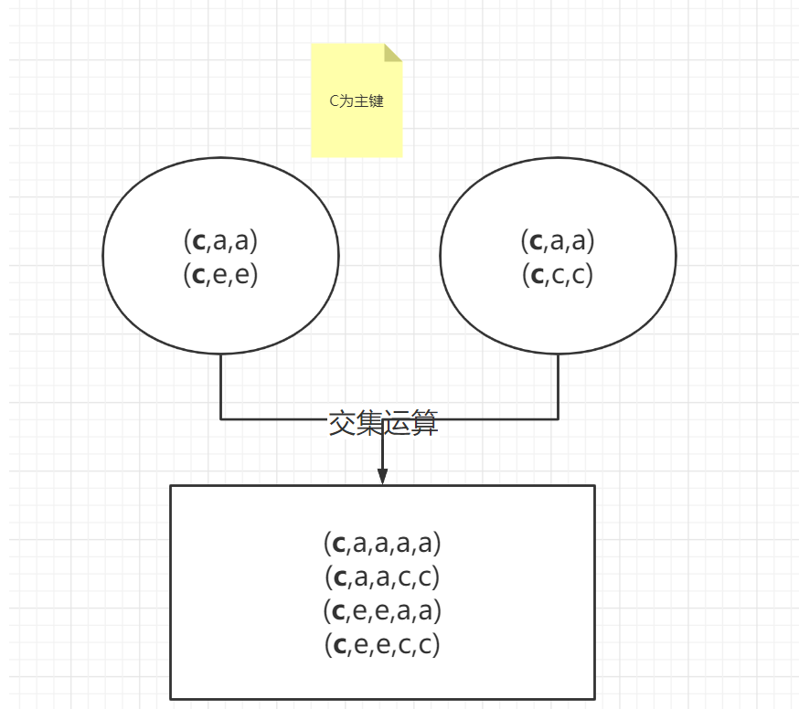
left = pd.DataFrame(
    {'key':['c','d','c'],
    'A':['a','b','e'],
    'B':['a','b','e']},
)
right = pd.DataFrame(
    {'key':['c','d','c'],
    'C':['a','b','c'],
    'D':['a','b','c']},
)

left

	key	A	B
0	c	a	a
1	d	b	b
2	c	e	e

right

	key	C	D
0	c	a	a
1	d	b	b
2	c	c	c

pd.merge(left,right,on=['key'])

	key	A	B	C	D
0	c	a	a	a	a
1	c	a	a	c	c
2	c	e	e	a	a
3	c	e	e	c	c
4	d	b	b	b	b

left = pd.DataFrame({'key1': ['K0', 'K0', 'K1', 'K2'],
                    'key2': ['K0', 'K1', 'K0', 'K1'],
                    'A': ['A0', 'A1', 'A2', 'A3'],
                    'B': ['B0', 'B1', 'B2', 'B3']})
right = pd.DataFrame({'key1': ['K0', 'K1', 'K1', 'K2'],
                      'key2': ['K0', 'K0', 'K0', 'K0'],
                      'C': ['C0', 'C1', 'C2', 'C3'],
                      'D': ['D0', 'D1', 'D2', 'D3']})
print(pd.merge(left, right, how='left', on=['key1', 'key2']))

## Match all key pairs in the left data frame. If right is not available, it will not match.

  key1 key2    A    B   C   D
0   K0   K0   A0   B0  C0  D0
1   K1   K0   A2   B2  C1  D1
2   K1   K0   A2   B2  C2  D2
3   K2   K0  NaN  NaN  C3  D3

print(pd.merge(left, right, how='right', on=['key1', 'key2']))

## Match all key pairs in the right data frame. If there is no left, it will not match.

  key1 key2    A    B   C   D
0   K0   K0   A0   B0  C0  D0
1   K1   K0   A2   B2  C1  D1
2   K1   K0   A2   B2  C2  D2
3   K2   K0  NaN  NaN  C3  D3

External connection, all values. If they do not exist, fill them with na (Union)

left = pd.DataFrame({'key1': ['K0', 'K0', 'K1', 'K2'],
                    'key2': ['K0', 'K1', 'K0', 'K1'],
                    'A': ['A0', 'A1', 'A2', 'A3'],
                    'B': ['B0', 'B1', 'B2', 'B3']})
right = pd.DataFrame({'key1': ['K0', 'K1', 'K1', 'K2'],
                      'key2': ['K0', 'K0', 'K0', 'K0'],
                      'C': ['C0', 'C1', 'C2', 'C3'],
                      'D': ['D0', 'D1', 'D2', 'D3']})
print(pd.merge(left,right,how='outer',on=['key1','key2']))

  key1 key2    A    B    C    D
0   K0   K0   A0   B0   C0   D0
1   K0   K1   A1   B1  NaN  NaN
2   K1   K0   A2   B2   C1   D1
3   K1   K0   A2   B2   C2   D2
4   K2   K1   A3   B3  NaN  NaN
5   K2   K0  NaN  NaN   C3   D3

Process column name duplicates

# Process duplicate column names
df_obj1 = pd.DataFrame({'key': ['b', 'b', 'a', 'c', 'a', 'a', 'b'],
                        'data' : np.random.randint(0,10,7)})
df_obj2 = pd.DataFrame({'key': ['a', 'b', 'd'],
                        'data' : np.random.randint(0,10,3)})

df_obj1

	key	data
0	b	4
1	b	5
2	a	3
3	c	0
4	a	4
5	a	5
6	b	4

df_obj2

	key	data
0	a	8
1	b	7
2	d	8

print(pd.merge(df_obj1, df_obj2, on='key', suffixes=('_left', '_right')))

  key  data_left  data_right
0   b          4           7
1   b          5           7
2   b          4           7
3   a          3           8
4   a          4           8
5   a          5           8

# Connect by index
df_obj1 = pd.DataFrame({'key': ['b', 'b', 'a', 'c', 'a', 'a', 'b'],
                        'data1' : np.random.randint(0,10,7)})
df_obj2 = pd.DataFrame({'data2' : np.random.randint(0,10,3)}, index=['a', 'b', 'd'])

  key  data1  data2
0   b      4      8
1   b      0      8
6   b      1      8
2   a      6      1
4   a      4      1
5   a      2      1

df_obj1

	key	data1
0	b	4
1	b	0
2	a	6
3	c	1
4	a	4
5	a	2
6	b	1

df_obj2

	data2
a	1
b	8
d	8

# It refers to the connection by index with the left key as the primary key.
pd.merge(df_obj1, df_obj2, left_on='key', right_index=True)

	key	data1	data2
0	b	4	8
1	b	0	8
6	b	1	8
2	a	6	1
4	a	4	1
5	a	2	1

pd.concat() method

Similar to np.concat, connect arrays. Here, connect dataframe s.

df1 = pd.DataFrame(np.arange(6).reshape(3,2),index=list('abc'),columns=['one','two'])

df2 = pd.DataFrame(np.arange(4).reshape(2,2)+5,index=list('ac'),columns=['three','four'])

df1

	one	two
a	0	1
b	2	3
c	4	5

df2

	three	four
a	5	6
c	7	8

## The default connection method is external connection, which is called Union.
pd.concat([df1,df2])

	one	two	three	four
a	0.0	1.0	NaN	NaN
b	2.0	3.0	NaN	NaN
c	4.0	5.0	NaN	NaN
a	NaN	NaN	5.0	6.0
c	NaN	NaN	7.0	8.0

## Of course, as in the previous methods, you can specify the parameter axis, which is similar to the above operation. merge() method
pd.concat([df1,df2],axis=1)

	one	two	three	four
a	0	1	5.0	6.0
b	2	3	NaN	NaN
c	4	5	7.0	8.0

## Similarly, you can also specify the connection method, such as the connection (intersection) in 'inner'
pd.concat([df1,df2],axis=1,join='inner')

	one	two	three	four
a	0	1	5	6
c	4	5	7	8

Reshaping data

# 1. Convert column index to row index: stack method
df_obj = pd.DataFrame(np.random.randint(0,10, (5,2)), columns=['data1', 'data2'])

stacked = df_obj.stack()

   data1  data2
0      5      3
1      7      4
2      5      7
3      7      2
4      9      5
0  data1    5
   data2    3
1  data1    7
   data2    4
2  data1    5
   data2    7
3  data1    7
   data2    2
4  data1    9
   data2    5
dtype: int32

df_obj

	data1	data2
0	5	3
1	7	4
2	5	7
3	7	2
4	9	5

stacked

0  data1    5
   data2    3
1  data1    7
   data2    4
2  data1    5
   data2    7
3  data1    7
   data2    2
4  data1    9
   data2    5
dtype: int32

As above, the data index becomes a hierarchical index.

print(type(df_obj))
# You can see that the data format has changed from dataframe to series
print(type(stacked))

<class 'pandas.core.frame.DataFrame'>
<class 'pandas.core.series.Series'>

# 2. Expand the hierarchical index to the row index unstack() method
stacked.unstack()

	data1	data2
0	5	3
1	7	4
2	5	7
3	7	2
4	9	5

Sort it out as a whole.

Why data cleaning? It is for the convenience of subsequent data analysis, modeling and other operations.
Which step is data cleaning in data analysis? Serve for data analysis and model before data analysis.
Data cleaning process?
It is divided into several categories:

1. Processing missing values
2. Repeat value processing
3. Data format conversion
4. Data consolidation

ok, that's it today. I'm not going to write a blog specifically for the time series structure, so I intend to directly infiltrate it into the later actual combat. Before the actual combat, I need to add some statistical knowledge. Thank you for your attention. Students who study python can use wechat as a blogger to communicate directly if they have questions.