Catalog
1sgd (random gradient descent) method
5.1.6,common/multi_layer_net.py
1 ch06/optimizer_compare_mnist
5.4 realization of four gradient optimization paths
This article is a summary of the introduction to deep learning theory and Implementation Based on Python. The author is [RI] Saito KANGYI
This paper mainly deals with
1. Find the optimization method with the most weight parameters, the initial value of the weight parameters, and the setting method of the super parameters.
2 prevent over fitting (weight attenuation, Dropout)
Introduction to 3 batch normalization
Parameter update
The purpose of neural network learning is to find the parameters that make the value of loss function as small as possible. This is the problem of finding the optimal parameters. The process of solving this problem is called optimization.
In the previous code implementation, in order to find the optimal parameter, the gradient (derivative) of the parameter is taken as the clue. Using the gradient of the parameter, update the parameter along the gradient direction, and repeat this step many times, so as to gradually approach the optimal parameter. This process is called the stochastic gradient descent (SGD).
When a person wants to go from the top to the bottom of the mountain, he will always find the fastest path. How to choose this path is the method to be discussed?
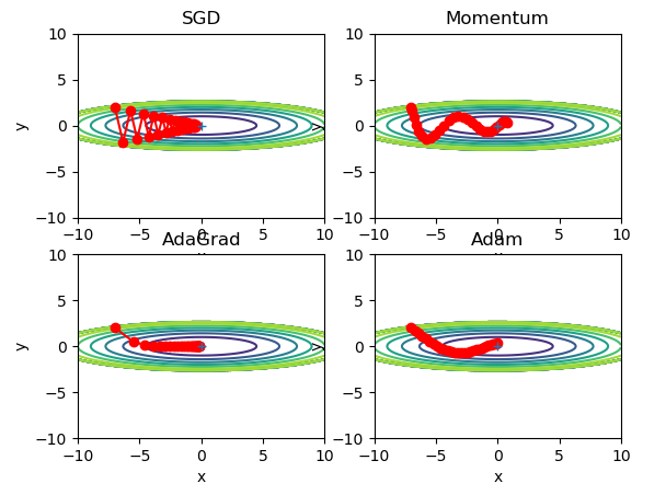
The four optimal paths of the gradient method are as follows: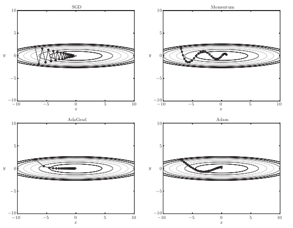
1sgd (random gradient descent) method
In fact, the update of gradient is the update of weight. SGD formula is obtained:

[note] record the weight parameter to be updated as W, and the gradient of loss function with respect to w as
η is the learning rate, which is actually 0.01 or 0.001.
The code implementation is as follows:
class SGD:
    def __init__(self, lr=0.01):
        self.lr = lr
        self.params = {}
        self.params['W1'] = 1
        self.params['b1'] = 2

    def update(self, params, grads):
        for key in params.keys():
            params[key] -= self.lr * grads[key]

        return params


if __name__ == "__main__":

    sgd = SGD()
    grads = {'W1': 0.1, 'b1': 0.3}
    r = sgd.update(sgd.params, grads)  # {'W1': 0.999, 'b1': 1.997}
1.1SGD drawback
SGD is simple and easy to implement, but it may not be efficient in solving some problems. See the following formula:

Its image is:
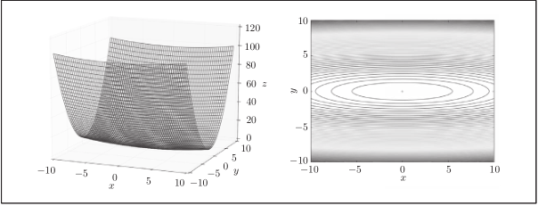
[note] image and contour
The gradient image is: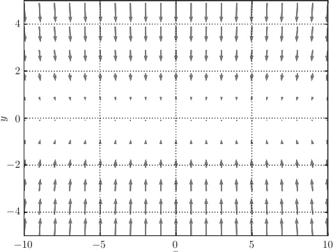
[note] although the minimum value of f(x,y) is at (x, y) = (0, 0), the gradient in the above figure does not point to (0, 0) in many places.
For example, search from (x, y) = (− 7.0, 2.0) (initial value), and the results are shown in the following figure.
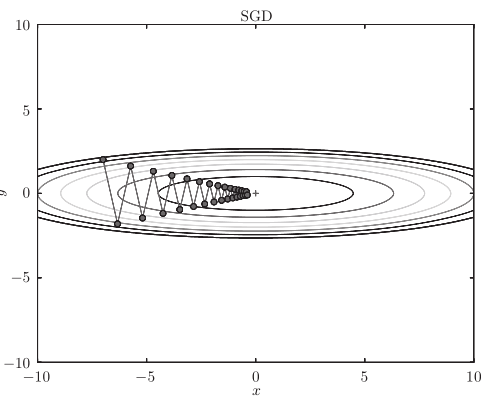
[note] SGD moves in zigzag shape. This is a rather inefficient path. In other words, the disadvantage of SGD is that if the shape of the function is non-uniform, such as extended, the search path will be very inefficient. The root cause of SGD inefficiency is that the direction of gradient does not point to the direction of minimum value.
2Momentum method
Momentum means "momentum". The formula is as follows: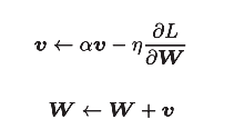
[note] like the previous SGD, W represents the weight parameter to be updated,  Represents the gradient of loss function with respect to W, and η represents the learning rate. Here we have a new variable v, which corresponds to the physical velocity. The first formula represents the physical law that the object is forced in the direction of gradient, under the action of which the speed of the object increases. The Momentum method feels like a ball rolling on the ground. The following picture:
[note] there is a term α v in the formula. When the object is free of any force, this task is to slow down the object gradually (α is set to a value of 0.9, etc.), corresponding to the physical ground friction or air resistance.
The optimized path is as follows: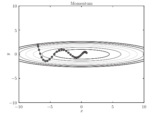
Note: the update path is like a ball rolling in a bowl. Compared with SGD, we find that the "degree" of zigzag is reduced. This is because although the force in the x-axis direction is very small, it is always in the same direction, so there will be some acceleration in the same direction. On the other hand, although the force on the y-axis is very large, the velocity on the y-axis is not stable because the forces on the positive and the negative directions are mutually offset. Therefore, compared with the case of SGD, it can approach to the x-axis faster and reduce the change of zigzag.
The code implementation is as follows:
import numpy as np

class Momentum:
    def __init__(self, lr=0.01, momentum=0.9):
        self.lr = lr
        self.momentum = momentum
        self.v = None

    def update(self, params, grads):
        if self.v is None:
            self.v = {}
            for key, val in params.items():
                self.v[key] = np.zeros_like(val)

        for key in params.keys():
            self.v[key] = self.momentum * self.v[key] - self.lr * grads[key]
            params[key] += self.v[key]
3AdaGrad method
In the learning of neural network, the value of learning rate (η in mathematical formula) is very important. If the learning rate is too small, it will cost too much time; conversely, if the learning rate is too large, it will lead to learning divergence and can not be carried out correctly.
Among the effective skills about learning rate, there is a method called learning rate decay, that is, with the progress of learning, the learning rate gradually decreases. In fact, the method of "more" learning and "less" learning is often used in neural network learning
The mathematical formula is as follows: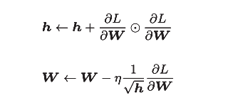
[note] like the previous SGD, W represents the weight parameter to be updated, Represents the gradient of loss function with respect to W, and η represents the learning rate. The new variable h, as shown in the first formula, holds the sum of squares of all previous gradient values
 Represents the multiplication of the corresponding matrix elements). Then, when updating the parameters, you can adjust the learning scale by multiplying by 1/sqrt(h).
This means that the learning rate of the elements with larger changes (greatly updated) in the parameters will be smaller. In other words, the learning rate can be attenuated according to the elements of the parameters, so that the learning rate of the parameters with large changes can be gradually reduced.
The code implementation is as follows:
# That is to say, with the progress of learning, the learning rate gradually decreases.
class AdaGrad:
    def __init__(self, lr=0.01):
        self.lr = lr
        self.h = None

    def update(self, params, grads):
        if self.h is None:
            self.h = {}
            for key, val in params.items():
                self.h[key] = np.zeros_like(val)

        for key in params.keys():
            self.h[key] += grads[key] * grads[key]
            params[key] -= self.lr * grads[key]/(np.sqrt(self.h[key]) + 1e-7)
The optimization path is as follows:
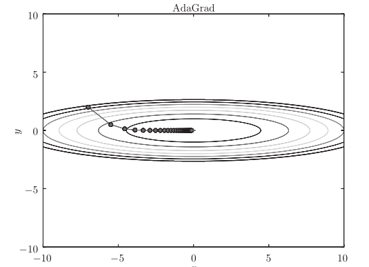
[note] from the above figure, the value of the function moves to the minimum value efficiently. Since the gradient in the y-axis direction is large, the change is large at the beginning, but it will be adjusted in proportion according to the large change later to reduce the update pace. Therefore, the degree of updating in the y-axis direction is weakened, and the change degree of zigzag is decreased.
4Adam method
By combining the two methods of Momentum and AdaGrad, we can achieve efficient search and "offset correction" of super parameters.
The mathematical formula is as follows:
[note] Adam will set three super parameters. One is the learning rate (in the paper, it appears as α), the other two are the primary momentum coefficient β 1 and the secondary momentum coefficient β 2. According to the paper, the standard setting value is 0.9 for β 1 and 0.999 for β 2. When these values are set, it will run smoothly in most cases.
The optimization path is as follows:
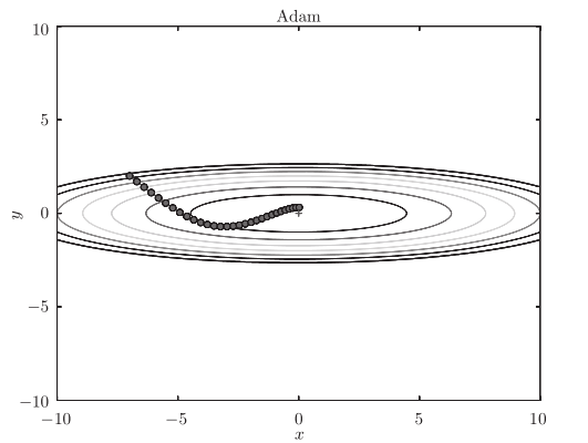
[note] the update process based on Adam is like a ball rolling in a bowl. Although momentum has a similar movement, Adam's ball, by contrast, wobbles to the left and right
Some reduction. This is because the degree of renewal of learning has been properly adjusted.
import numpy as np

class Adam:

    def __init__(self, lr=0.001, beta1=0.9, beta2=0.999):
        self.lr = lr
        self.beta1 = beta1
        self.beta2 = beta2
        self.iter = 0
        self.m = None
        self.v = None

    def update(self, params, grads):
        if self.m is None:
            self.m, self.v = {}, {}
            for key, val in params.items():
                self.m[key] = np.zeros_like(val)
                self.v[key] = np.zeros_like(val)

        self.iter += 1
        lr_t = self.lr * np.sqrt(1.0 - self.beta2 ** self.iter) / (1.0 - self.beta1 ** self.iter)

        for key in params.keys():
            self.m[key] += (1 - self.beta1) * (grads[key] - self.m[key])
            self.v[key] += (1 - self.beta2) * (grads[key] ** 2 - self.v[key])

            params[key] -= lr_t * self.m[key] / (np.sqrt(self.v[key]) + 1e-7)
5 cases
Case: comparison of update methods based on MNIST dataset
The contents are as follows: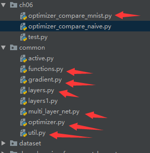
5.1 common folder
5.1.1,common/functions.py
import numpy as np


def sigmoid(x):
    return 1/(1 + np.exp(-x))


def sigmoid_grad(x):
    return (1.0 - sigmoid(x)) * sigmoid(x)


# Activation function of output layer
def softmax(x):
    if x.ndim == 2:
        x = x.T
        x = x - np.max(x, axis=0)
        y = np.exp(x)/np.sum(np.exp(x), axis=0)
        return y.T

    x = x - np.max(x, axis=0)
    return np.exp(x)/np.sum(np.exp(x))


# Cross entropy error
def cross_entropy_error(y, t):
    if y.ndim == 1:
        t = t.reshape(1, t.size)
        y = y.reshape(1, y.size)

    if y.size == t.size:
        t = t.argmax(axis=1)

    batch_size = y.shape[0]
    return -np.sum(np.log(y[np.arange(batch_size), t] + 1e-7))/batch_size
5.1.2,common/gradient.py
import numpy as np


def numerical_gradient(f, x):
    h = 1e-4
    grad = np.zeros_like(x)  # Construct the same dimension
    # By default, nditer treats the array to be iterated as read-only
    # In order to traverse the array and modify the array element value, you must specify the op'flags = ['readwrite '] mode:
    it = np.nditer(x, flags=['multi_index'], op_flags=['readwrite'])
    # Row traversal of array x
    while not it.finished:
        idx = it.multi_index  # Indexes
        tmp_val = x[idx]
        x[idx] = tmp_val + h
        fxh1 = f(x)

        x[idx] = tmp_val - h
        fxh2 = f(x)

        grad[idx] = (fxh1 - fxh2)/2*h

        x[idx] = tmp_val
        it.iternext()
    return grad
5.1.3,common/layers.py
# coding: utf-8
import numpy as np
from common.functions import *
from common.util import im2col, col2im


class Relu:
    def __init__(self):
        self.mask = None

    def forward(self, x):
        self.mask = (x <= 0)
        out = x.copy()
        out[self.mask] = 0

        return out

    def backward(self, dout):
        dout[self.mask] = 0
        dx = dout

        return dx


class Sigmoid:
    def __init__(self):
        self.out = None

    def forward(self, x):
        out = sigmoid(x)
        self.out = out
        return out

    def backward(self, dout):
        dx = dout * (1.0 - self.out) * self.out

        return dx


class Affine:
    def __init__(self, W, b):
        self.W =W
        self.b = b

        self.x = None
        self.original_x_shape = None
        #
        self.dW = None
        self.db = None

    def forward(self, x):
        #
        self.original_x_shape = x.shape
        x = x.reshape(x.shape[0], -1)
        self.x = x

        out = np.dot(self.x, self.W) + self.b

        return out

    def backward(self, dout):
        dx = np.dot(dout, self.W.T)
        self.dW = np.dot(self.x.T, dout)
        self.db = np.sum(dout, axis=0)

        dx = dx.reshape(*self.original_x_shape)  #
        return dx


class SoftmaxWithLoss:
    def __init__(self):
        self.loss = None
        self.y = None #
        self.t = None #

    def forward(self, x, t):
        self.t = t
        self.y = softmax(x)
        self.loss = cross_entropy_error(self.y, self.t)

        return self.loss

    def backward(self, dout=1):
        batch_size = self.t.shape[0]
        if self.t.size == self.y.size:
            dx = (self.y - self.t) / batch_size
        else:
            dx = self.y.copy()
            dx[np.arange(batch_size), self.t] -= 1
            dx = dx / batch_size

        return dx


class Dropout:
    """
    http://arxiv.org/abs/1207.0580
    """
    def __init__(self, dropout_ratio=0.5):
        self.dropout_ratio = dropout_ratio
        self.mask = None

    def forward(self, x, train_flg=True):
        if train_flg:
            self.mask = np.random.rand(*x.shape) > self.dropout_ratio
            return x * self.mask
        else:
            return x * (1.0 - self.dropout_ratio)

    def backward(self, dout):
        return dout * self.mask


class BatchNormalization:
    """
    http://arxiv.org/abs/1502.03167
    """
    def __init__(self, gamma, beta, momentum=0.9, running_mean=None, running_var=None):
        self.gamma = gamma
        self.beta = beta
        self.momentum = momentum
        self.input_shape = None #

        #
        self.running_mean = running_mean
        self.running_var = running_var

        #
        self.batch_size = None
        self.xc = None
        self.std = None
        self.dgamma = None
        self.dbeta = None

    def forward(self, x, train_flg=True):
        self.input_shape = x.shape
        if x.ndim != 2:
            N, C, H, W = x.shape
            x = x.reshape(N, -1)

        out = self.__forward(x, train_flg)

        return out.reshape(*self.input_shape)

    def __forward(self, x, train_flg):
        if self.running_mean is None:
            N, D = x.shape
            self.running_mean = np.zeros(D)
            self.running_var = np.zeros(D)

        if train_flg:
            mu = x.mean(axis=0)
            xc = x - mu
            var = np.mean(xc**2, axis=0)
            std = np.sqrt(var + 10e-7)
            xn = xc / std

            self.batch_size = x.shape[0]
            self.xc = xc
            self.xn = xn
            self.std = std
            self.running_mean = self.momentum * self.running_mean + (1-self.momentum) * mu
            self.running_var = self.momentum * self.running_var + (1-self.momentum) * var
        else:
            xc = x - self.running_mean
            xn = xc / ((np.sqrt(self.running_var + 10e-7)))

        out = self.gamma * xn + self.beta
        return out

    def backward(self, dout):
        if dout.ndim != 2:
            N, C, H, W = dout.shape
            dout = dout.reshape(N, -1)

        dx = self.__backward(dout)

        dx = dx.reshape(*self.input_shape)
        return dx

    def __backward(self, dout):
        dbeta = dout.sum(axis=0)
        dgamma = np.sum(self.xn * dout, axis=0)
        dxn = self.gamma * dout
        dxc = dxn / self.std
        dstd = -np.sum((dxn * self.xc) / (self.std * self.std), axis=0)
        dvar = 0.5 * dstd / self.std
        dxc += (2.0 / self.batch_size) * self.xc * dvar
        dmu = np.sum(dxc, axis=0)
        dx = dxc - dmu / self.batch_size

        self.dgamma = dgamma
        self.dbeta = dbeta

        return dx


class Convolution:
    def __init__(self, W, b, stride=1, pad=0):
        self.W = W
        self.b = b
        self.stride = stride
        self.pad = pad

        #
        self.x = None
        self.col = None
        self.col_W = None

        #
        self.dW = None
        self.db = None

    def forward(self, x):
        FN, C, FH, FW = self.W.shape
        N, C, H, W = x.shape
        out_h = 1 + int((H + 2*self.pad - FH) / self.stride)
        out_w = 1 + int((W + 2*self.pad - FW) / self.stride)

        col = im2col(x, FH, FW, self.stride, self.pad)
        col_W = self.W.reshape(FN, -1).T

        out = np.dot(col, col_W) + self.b
        out = out.reshape(N, out_h, out_w, -1).transpose(0, 3, 1, 2)

        self.x = x
        self.col = col
        self.col_W = col_W

        return out

    def backward(self, dout):
        FN, C, FH, FW = self.W.shape
        dout = dout.transpose(0,2,3,1).reshape(-1, FN)

        self.db = np.sum(dout, axis=0)
        self.dW = np.dot(self.col.T, dout)
        self.dW = self.dW.transpose(1, 0).reshape(FN, C, FH, FW)

        dcol = np.dot(dout, self.col_W.T)
        dx = col2im(dcol, self.x.shape, FH, FW, self.stride, self.pad)

        return dx


class Pooling:
    def __init__(self, pool_h, pool_w, stride=1, pad=0):
        self.pool_h = pool_h
        self.pool_w = pool_w
        self.stride = stride
        self.pad = pad

        self.x = None
        self.arg_max = None

    def forward(self, x):
        N, C, H, W = x.shape
        out_h = int(1 + (H - self.pool_h) / self.stride)
        out_w = int(1 + (W - self.pool_w) / self.stride)

        col = im2col(x, self.pool_h, self.pool_w, self.stride, self.pad)
        col = col.reshape(-1, self.pool_h*self.pool_w)

        arg_max = np.argmax(col, axis=1)
        out = np.max(col, axis=1)
        out = out.reshape(N, out_h, out_w, C).transpose(0, 3, 1, 2)

        self.x = x
        self.arg_max = arg_max

        return out

    def backward(self, dout):
        dout = dout.transpose(0, 2, 3, 1)

        pool_size = self.pool_h * self.pool_w
        dmax = np.zeros((dout.size, pool_size))
        dmax[np.arange(self.arg_max.size), self.arg_max.flatten()] = dout.flatten()
        dmax = dmax.reshape(dout.shape + (pool_size,))

        dcol = dmax.reshape(dmax.shape[0] * dmax.shape[1] * dmax.shape[2], -1)
        dx = col2im(dcol, self.x.shape, self.pool_h, self.pool_w, self.stride, self.pad)

        return dx
5.1.4,common/util.py
# coding: utf-8
import numpy as np


def smooth_curve(x):

    window_len = 11
    s = np.r_[x[window_len-1:0:-1], x, x[-1:-window_len:-1]]
    w = np.kaiser(window_len, 2)
    y = np.convolve(w/w.sum(), s, mode='valid')
    return y[5:len(y)-5]


def shuffle_dataset(x, t):
    permutation = np.random.permutation(x.shape[0])
    x = x[permutation,:] if x.ndim == 2 else x[permutation,:,:,:]
    t = t[permutation]

    return x, t

def conv_output_size(input_size, filter_size, stride=1, pad=0):
    return (input_size + 2*pad - filter_size) / stride + 1


def im2col(input_data, filter_h, filter_w, stride=1, pad=0):
    N, C, H, W = input_data.shape
    out_h = (H + 2*pad - filter_h)//stride + 1
    out_w = (W + 2*pad - filter_w)//stride + 1

    img = np.pad(input_data, [(0,0), (0,0), (pad, pad), (pad, pad)], 'constant')
    col = np.zeros((N, C, filter_h, filter_w, out_h, out_w))

    for y in range(filter_h):
        y_max = y + stride*out_h
        for x in range(filter_w):
            x_max = x + stride*out_w
            col[:, :, y, x, :, :] = img[:, :, y:y_max:stride, x:x_max:stride]

    col = col.transpose(0, 4, 5, 1, 2, 3).reshape(N*out_h*out_w, -1)
    return col


def col2im(col, input_shape, filter_h, filter_w, stride=1, pad=0):
    N, C, H, W = input_shape
    out_h = (H + 2*pad - filter_h)//stride + 1
    out_w = (W + 2*pad - filter_w)//stride + 1
    col = col.reshape(N, out_h, out_w, C, filter_h, filter_w).transpose(0, 3, 4, 5, 1, 2)

    img = np.zeros((N, C, H + 2*pad + stride - 1, W + 2*pad + stride - 1))
    for y in range(filter_h):
        y_max = y + stride*out_h
        for x in range(filter_w):
            x_max = x + stride*out_w
            img[:, :, y:y_max:stride, x:x_max:stride] += col[:, :, y, x, :, :]

    return img[:, :, pad:H + pad, pad:W + pad]
5.1.5,common/optimizer.py
import numpy as np


class SGD:
    def __init__(self, lr=0.01):
        self.lr = lr
        self.params = {}
        self.params['b1'] = 1
        self.params['b2'] = 2

    def update(self, params, grads):
        for key in params.keys():
            params[key] -= self.lr * grads[key]

        return params


class Momentum:
    def __init__(self, lr=0.01, momentum=0.9):
        self.lr = lr
        self.momentum = momentum
        self.v = None

    def update(self, params, grads):
        if self.v is None:
            self.v = {}
            for key, val in params.items():
                self.v[key] = np.zeros_like(val)

        for key in params.keys():
            self.v[key] = self.momentum * self.v[key] - self.lr * grads[key]
            params[key] += self.v[key]


# That is to say, with the progress of learning, the learning rate gradually decreases.
class AdaGrad:
    def __init__(self, lr=0.01):
        self.lr = lr
        self.h = None

    def update(self, params, grads):
        if self.h is None:
            self.h = {}
            for key, val in params.items():
                self.h[key] = np.zeros_like(val)

        for key in params.keys():
            self.h[key] += grads[key] * grads[key]
            params[key] -= self.lr * grads[key]/(np.sqrt(self.h[key]) + 1e-7)


class Adam:

    def __init__(self, lr=0.001, beta1=0.9, beta2=0.999):
        self.lr = lr
        self.beta1 = beta1
        self.beta2 = beta2
        self.iter = 0
        self.m = None
        self.v = None

    def update(self, params, grads):
        if self.m is None:
            self.m, self.v = {}, {}
            for key, val in params.items():
                self.m[key] = np.zeros_like(val)
                self.v[key] = np.zeros_like(val)

        self.iter += 1
        lr_t = self.lr * np.sqrt(1.0 - self.beta2 ** self.iter) / (1.0 - self.beta1 ** self.iter)

        for key in params.keys():
            self.m[key] += (1 - self.beta1) * (grads[key] - self.m[key])
            self.v[key] += (1 - self.beta2) * (grads[key] ** 2 - self.v[key])

            params[key] -= lr_t * self.m[key] / (np.sqrt(self.v[key]) + 1e-7)
5.1.6,common/multi_layer_net.py
# coding: utf-8
import sys, os
sys.path.append(os.pardir)  #
import numpy as np
from collections import OrderedDict
from common.layers import *
from common.gradient import numerical_gradient


class MultiLayerNet:

    def __init__(self, input_size, hidden_size_list, output_size,
                 activation='relu', weight_init_std='relu', weight_decay_lambda=0):
        self.input_size = input_size
        self.output_size = output_size
        self.hidden_size_list = hidden_size_list
        self.hidden_layer_num = len(hidden_size_list)
        self.weight_decay_lambda = weight_decay_lambda
        self.params = {}

        #
        self.__init_weight(weight_init_std)

        #
        activation_layer = {'sigmoid': Sigmoid, 'relu': Relu}
        self.layers = OrderedDict()
        for idx in range(1, self.hidden_layer_num+1):
            self.layers['Affine' + str(idx)] = Affine(self.params['W' + str(idx)],
                                                      self.params['b' + str(idx)])
            self.layers['Activation_function' + str(idx)] = activation_layer[activation]()

        idx = self.hidden_layer_num + 1
        self.layers['Affine' + str(idx)] = Affine(self.params['W' + str(idx)],
            self.params['b' + str(idx)])

        self.last_layer = SoftmaxWithLoss()

    def __init_weight(self, weight_init_std):

        all_size_list = [self.input_size] + self.hidden_size_list + [self.output_size]
        for idx in range(1, len(all_size_list)):
            scale = weight_init_std
            if str(weight_init_std).lower() in ('relu', 'he'):
                scale = np.sqrt(2.0 / all_size_list[idx - 1])  #
            elif str(weight_init_std).lower() in ('sigmoid', 'xavier'):
                scale = np.sqrt(1.0 / all_size_list[idx - 1])  #

            self.params['W' + str(idx)] = scale * np.random.randn(all_size_list[idx-1], all_size_list[idx])
            self.params['b' + str(idx)] = np.zeros(all_size_list[idx])

    def predict(self, x):
        for layer in self.layers.values():
            x = layer.forward(x)

        return x

    def loss(self, x, t):
        y = self.predict(x)

        weight_decay = 0
        for idx in range(1, self.hidden_layer_num + 2):
            W = self.params['W' + str(idx)]
            weight_decay += 0.5 * self.weight_decay_lambda * np.sum(W ** 2)

        return self.last_layer.forward(y, t) + weight_decay

    def accuracy(self, x, t):
        y = self.predict(x)
        y = np.argmax(y, axis=1)
        if t.ndim != 1 : t = np.argmax(t, axis=1)

        accuracy = np.sum(y == t) / float(x.shape[0])
        return accuracy

    def numerical_gradient(self, x, t):
        loss_W = lambda W: self.loss(x, t)

        grads = {}
        for idx in range(1, self.hidden_layer_num+2):
            grads['W' + str(idx)] = numerical_gradient(loss_W, self.params['W' + str(idx)])
            grads['b' + str(idx)] = numerical_gradient(loss_W, self.params['b' + str(idx)])

        return grads

    def gradient(self, x, t):
        # forward
        self.loss(x, t)

        # backward
        dout = 1
        dout = self.last_layer.backward(dout)

        layers = list(self.layers.values())
        layers.reverse()
        for layer in layers:
            dout = layer.backward(dout)

        #
        grads = {}
        for idx in range(1, self.hidden_layer_num+2):
            grads['W' + str(idx)] = self.layers['Affine' + str(idx)].dW + self.weight_decay_lambda * self.layers['Affine' + str(idx)].W
            grads['b' + str(idx)] = self.layers['Affine' + str(idx)].db

        return grads
5.2 ch06 folder
1 ch06/optimizer_compare_mnist
# coding: utf-8
import os
import sys
sys.path.append(os.pardir)  #
import matplotlib.pyplot as plt
from dataset.mnist import load_mnist
from common.util import smooth_curve
from common.multi_layer_net import MultiLayerNet
from common.optimizer import *


#
(x_train, t_train), (x_test, t_test) = load_mnist(normalize=True)

train_size = x_train.shape[0]
batch_size = 128
max_iterations = 2000


#
optimizers = {}
optimizers['SGD'] = SGD()
optimizers['Momentum'] = Momentum()
optimizers['AdaGrad'] = AdaGrad()
optimizers['Adam'] = Adam()
# optimizers['RMSprop'] = RMSprop()

networks = {}
train_loss = {}
for key in optimizers.keys():
    networks[key] = MultiLayerNet(
        input_size=784, hidden_size_list=[100, 100, 100, 100],
        output_size=10)
    train_loss[key] = []


# 2:
for i in range(max_iterations):
    batch_mask = np.random.choice(train_size, batch_size)
    x_batch = x_train[batch_mask]
    t_batch = t_train[batch_mask]

    for key in optimizers.keys():
        grads = networks[key].gradient(x_batch, t_batch)
        optimizers[key].update(networks[key].params, grads)

        loss = networks[key].loss(x_batch, t_batch)
        train_loss[key].append(loss)

    if i % 100 == 0:
        print( "===========" + "iteration:" + str(i) + "===========")
        for key in optimizers.keys():
            loss = networks[key].loss(x_batch, t_batch)
            print(key + ":" + str(loss))


# 3.
markers = {"SGD": "o", "Momentum": "x", "AdaGrad": "s", "Adam": "D"}
x = np.arange(max_iterations)
for key in optimizers.keys():
    plt.plot(x, smooth_curve(train_loss[key]), marker=markers[key], markevery=100, label=key)
plt.xlabel("iterations")
plt.ylabel("loss")
plt.ylim(0, 1)
plt.legend()
plt.show()
5.3 results
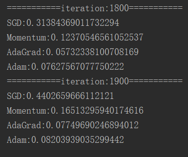
The results are as follows: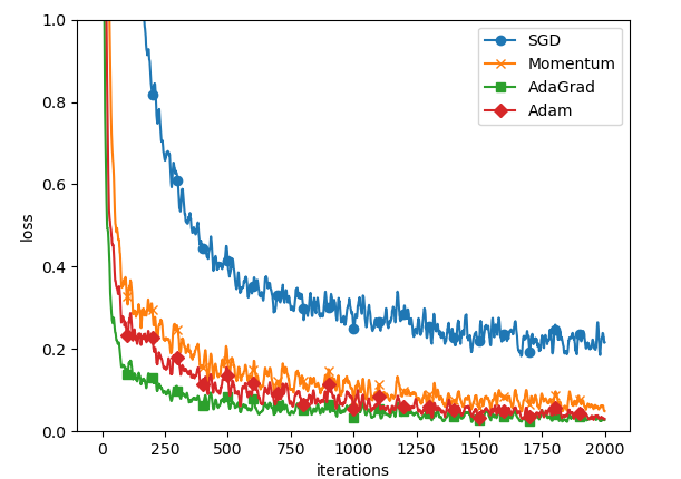
The comparison results are as follows:
5.4 realization of four gradient optimization paths
# coding: utf-8
import sys, os
sys.path.append(os.pardir)
import numpy as np
import matplotlib.pyplot as plt
from collections import OrderedDict
from common.optimizer import *


def f(x, y):
    return x**2 / 20.0 + y**2


def df(x, y):
    return x / 10.0, 2.0*y

# Initialization parameters
init_pos = (-7.0, 2.0)
params = {}
params['x'], params['y'] = init_pos[0], init_pos[1]
grads = {}
grads['x'], grads['y'] = 0, 0


# Implement sorting of elements in dictionary elements, (K, V)
optimizers = OrderedDict()
optimizers["SGD"] = SGD(lr=0.95)
optimizers["Momentum"] = Momentum(lr=0.1)
optimizers["AdaGrad"] = AdaGrad(lr=1.5)
optimizers["Adam"] = Adam(lr=0.3)

idx = 1

for key in optimizers:
    optimizer = optimizers[key]
    x_history = []
    y_history = []
    params['x'], params['y'] = init_pos[0], init_pos[1]

    for i in range(30):
        x_history.append(params['x'])
        y_history.append(params['y'])

        grads['x'], grads['y'] = df(params['x'], params['y'])
        optimizer.update(params, grads)

    x = np.arange(-10, 10, 0.01)
    y = np.arange(-5, 5, 0.01)

    # Convert vector to matrix
    X, Y = np.meshgrid(x, y)
    Z = f(X, Y)

    # for simple contour line
    mask = Z > 7
    Z[mask] = 0

    # plot
    plt.subplot(2, 2, idx)
    idx += 1
    plt.plot(x_history, y_history, 'o-', color="red")
    plt.contour(X, Y, Z)
    plt.ylim(-10, 10)
    plt.xlim(-10, 10)
    plt.plot(0, 0, '+')
    #colorbar()
    #spring()
    plt.title(key)
    plt.xlabel("x")
    plt.ylabel("y")

plt.show()
The operation results are as follows: