PixPro is the first to use pixel level contrast learning for feature representation learning
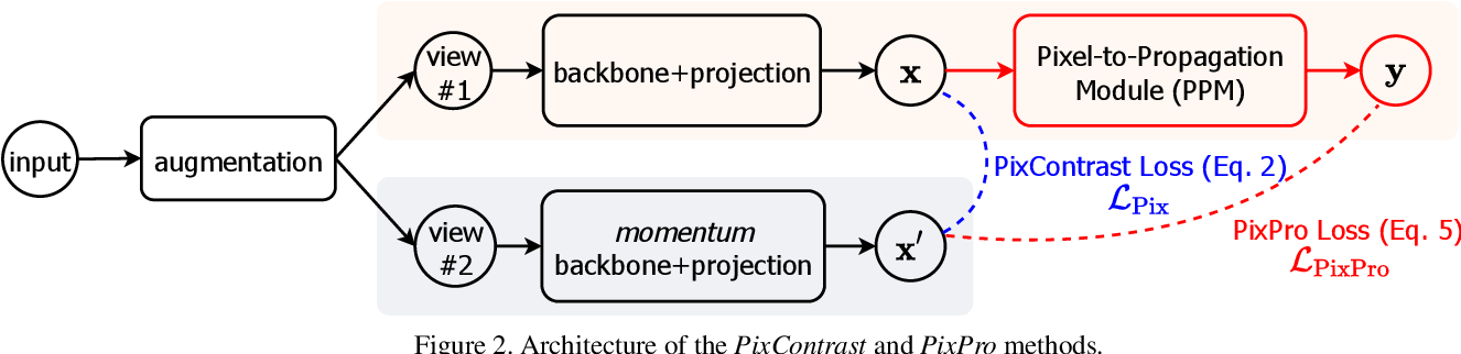
The above figure is the flow chart of the whole algorithm, which will be analyzed in detail next
Forward propagation
Input is the input image, and the dimension size is (b, c, h, w)
augmentation: cut the same input in random size and position and reduce it to the unified size 224 * 224, and perform random horizontal flip, color distortion, Gaussian blur and Solaris based on a certain probability. Finally, two different views view #1 and view #2 are generated, both of which are (b, c, 224, 224)
backbone+projection: view #1 and view #2 are sent to two network branches respectively. Both the upper and lower branches contain backbone+projection modules with the same structure. The backbone module uses Resnet to output the last layer of feature map with the size of (b, c1, 7, 7).
The projection module is a conv1*1+BN+Relu+conv1*1 structure. First upgrade the dimension and then reduce the dimension to 256. In this way, two features $x $and $x ^ {,} $with output size of (b, 256, 7, 7) are obtained. The code of the projection module is as follows:
class MLP2d(nn.Module):
    def __init__(self, in_dim, inner_dim=4096, out_dim=256):
        super(MLP2d, self).__init__()

        self.linear1 = conv1x1(in_dim, inner_dim)
        self.bn1 = nn.BatchNorm2d(inner_dim)
        self.relu1 = nn.ReLU(inplace=True)

        self.linear2 = conv1x1(inner_dim, out_dim)

    def forward(self, x):
        x = self.linear1(x)
        x = self.bn1(x)
        x = self.relu1(x)

        x = self.linear2(x)

        return x

def conv1x1(in_planes, out_planes):
    """1x1 convolution"""
    return nn.Conv2d(in_planes, out_planes, kernel_size=1, stride=1, padding=0, bias=True)
PPM: it is a self attention module. It is aimed at the input characteristic diagram $x of (b, 256, 7, 7)$
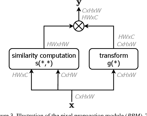
Firstly, the attention graph is calculated according to the cosine similarity, and the size is (b, 49, 49), indicating the similarity between each feature point and other feature points. Then feature fusion is performed on the input feature map to obtain the feature map $y $with the output size of (b, 256, 7, 7). The PPM code is as follows:
    def featprop(self, feat):
        N, C, H, W = feat.shape

        # Value transformation
        feat_value = self.value_transform(feat)  # 1 * 1 convolution operation
        feat_value = F.normalize(feat_value, dim=1)
        feat_value = feat_value.view(N, C, -1)

        # Similarity calculation
        feat = F.normalize(feat, dim=1)

        # [N, C, H * W]
        feat = feat.view(N, C, -1)

        # [N, H * W, H * W]
        attention = torch.bmm(feat.transpose(1, 2), feat)
        attention = torch.clamp(attention, min=self.pixpro_clamp_value)
        if self.pixpro_p < 1.:
            attention = attention + 1e-6
        attention = attention ** self.pixpro_p  # pixpro_p controls the range of attention. The default is 1

        # [N, C, H * W]
        feat = torch.bmm(feat_value, attention.transpose(1, 2))

        return feat.view(N, C, H, W)
Loss: calculate the loss between $x ^, $and $y $$ The spatial location diagram of x ^, $and $y $is as follows:
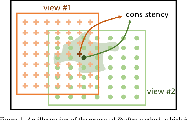
In the process of data enhancement augmentation, the coordinates of the upper left corner and the lower right key of the cropped image can be obtained. Since the size of the output feature map $x ^, $and $y $is (b, 256, 7, 7), there are 7 * 7 feature points in each feature map. According to the interpolation method, the spatial coordinates of each feature point of the output feature map $x ^, $and $y $can be obtained, and the size is (b, 2, 7, 7).
Firstly, the distance between each feature point in different views is calculated, and the distance matrix D with the size of (b, 49, 49) can be obtained. The steps are as follows:
- X coordinate of feature map $x ^ {,} $X_{x ^ {,}} $: (B, 7, 7) - > (B, 49, 1), y coordinate $Y_{x^{,}}$: (b, 7, 7)->(b, 49, 1)
- x coordinate in characteristic figure $y $$x_ {y} $: (B, 7, 7) - > (B, 1, 49), y coordinate $Y_{y}$: (b, 7, 7)->(b, 1,49)
- Distance matrix D = $\ sqrt {(x {x ^ {,}} - x {y}) ^ 2 + (Y {x ^ {,}} - y {y}) ^ 2} / Max\_ Bin $(max_bin is the maximum distance between adjacent feature points for "normalization")
The features of feature points closer in different views should have consistency, so the distance feature D is bisected according to the threshold ratio to obtain the mask of feature points closer M = (d < ratio)
Then calculate the feature similarity map logit of $x ^, $and $y $with the size of (b, 49, 49), which is similar to the calculation of attention similarity in PPM
Finally, loss is calculated according to the feature similarity diagram and mask matrix:
$loss = logit * M$
The code of the whole loss calculation process is as follows:
def regression_loss(q, k, coord_q, coord_k, pos_ratio=0.5):
    """ q, k: N * C * H * W
        coord_q, coord_k: N * 4 (x_upper_left, y_upper_left, x_lower_right, y_lower_right)
    """
    N, C, H, W = q.shape
    # [bs, feat_dim, 49]
    q = q.view(N, C, -1)
    k = k.view(N, C, -1)

    # generate center_coord, width, height
    # [1, 7, 7]
    x_array = torch.arange(0., float(W), dtype=coord_q.dtype, device=coord_q.device).view(1, 1, -1).repeat(1, H, 1)
    y_array = torch.arange(0., float(H), dtype=coord_q.dtype, device=coord_q.device).view(1, -1, 1).repeat(1, 1, W)
    # [bs, 1, 1]
    q_bin_width = ((coord_q[:, 2] - coord_q[:, 0]) / W).view(-1, 1, 1)
    q_bin_height = ((coord_q[:, 3] - coord_q[:, 1]) / H).view(-1, 1, 1)
    k_bin_width = ((coord_k[:, 2] - coord_k[:, 0]) / W).view(-1, 1, 1)
    k_bin_height = ((coord_k[:, 3] - coord_k[:, 1]) / H).view(-1, 1, 1)
    # [bs, 1, 1]
    q_start_x = coord_q[:, 0].view(-1, 1, 1)
    q_start_y = coord_q[:, 1].view(-1, 1, 1)
    k_start_x = coord_k[:, 0].view(-1, 1, 1)
    k_start_y = coord_k[:, 1].view(-1, 1, 1)

    # [bs, 1, 1]
    q_bin_diag = torch.sqrt(q_bin_width ** 2 + q_bin_height ** 2)
    k_bin_diag = torch.sqrt(k_bin_width ** 2 + k_bin_height ** 2)
    max_bin_diag = torch.max(q_bin_diag, k_bin_diag)

    # [bs, 7, 7]
    center_q_x = (x_array + 0.5) * q_bin_width + q_start_x
    center_q_y = (y_array + 0.5) * q_bin_height + q_start_y
    center_k_x = (x_array + 0.5) * k_bin_width + k_start_x
    center_k_y = (y_array + 0.5) * k_bin_height + k_start_y

    # [bs, 49, 49]
    dist_center = torch.sqrt((center_q_x.view(-1, H * W, 1) - center_k_x.view(-1, 1, H * W)) ** 2
                             + (center_q_y.view(-1, H * W, 1) - center_k_y.view(-1, 1, H * W)) ** 2) / max_bin_diag
    pos_mask = (dist_center < pos_ratio).float().detach()

    # [bs, 49, 49]
    logit = torch.bmm(q.transpose(1, 2), k)

    loss = (logit * pos_mask).sum(-1).sum(-1) / (pos_mask.sum(-1).sum(-1) + 1e-6)

    return -2 * loss.mean()
Back propagation
The lower branch network does not participate in direct training, and all weight parameters do not have gradient values. Its parameter $param\_ The K $update method is based on the upper branch network parameter $param\_q $momentum update. Before the training, the initial weights of the upper and lower branch networks remain the same.
$$ param\_k.data = param\_k.data * momentum + param\_q.data * (1-momentum) $$
Where momentum is the momentum value, which gradually increases from 0.99 to 1.0 in the whole training process
experiment
Optimizer: LARS, weight_decay=1e-5
lr_scheduler: cosine, warmup
total_batchsize: 1024
world size: 8 V100 GPUs
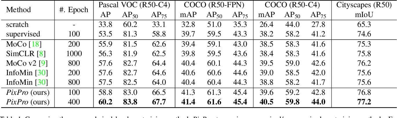
Comparison with other instance level self-monitoring algorithms in downstream detection and segmentation tasks
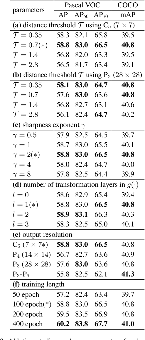
Experimental results under different super parameters
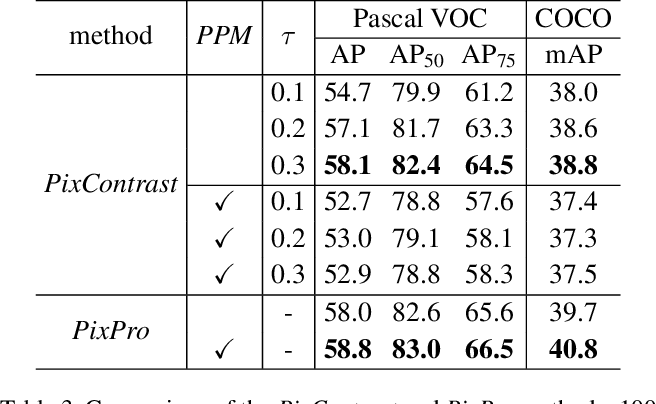
Comparison of PixPro and ProContrast results
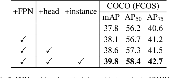
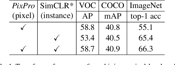
Combined with the results of instance level module
Whether there are experimental comparison results of FPN, head and instance level modules