Algorithm complexity

Complexity concept

The running time of the program needs to consume certain time resources and space (memory) resources. Therefore, the quality of an algorithm is generally measured from the two dimensions of time and space, namely time complexity and space complexity.

Time complexity mainly measures the running speed of an algorithm, while space complexity mainly measures the additional space required for the operation of an algorithm. In the early stage of computer development, the storage capacity of computer is very small, so it cares about space complexity. Nowadays, the storage capacity of computers has reached a high level, and there is no need to pay special attention to the spatial complexity of an algorithm.

Time complexity

Time complexity definition

The time complexity of the algorithm is a function, which quantitatively describes the running time of the algorithm. Theoretically, the specific time spent in the implementation of the algorithm can not be calculated, and even if the running time of the program is actually measured, the advantages and disadvantages of the algorithm can not be described for various reasons such as the performance of the machine.

Moreover, the machine calculation is too cumbersome, so there is the analysis method of time complexity. The time complexity does not calculate the specific time, but the execution times of the basic operations in the algorithm. Find a basic statement and the scale of the problem N N The mathematical expression between N is to calculate the time complexity of the algorithm.

Such as the following code: calculate the execution times of + + count statement in the code.

void Func(int N) {
	int count = 0;
	for (int i = 0; i < N; ++i) {
		for (int j = 0; j < N; ++j) {
			++count;
		}
	}
	for (int k = 0; k < 2 * N; ++k) {
		++count; 
    }
	int M = 10;
	while (M--) {
		++count;
        printf("hehe\n");
	}
}

From a mathematical point of view, the time complexity of the algorithm is actually a mathematical function about N, such as this problem F ( N ) = N 2 + 2 N + 10 F(N)=N^2+2N+10 F(N)=N2+2N+10.

Large O asymptotic representation

When N=10, F(N)=130, when N=100, F(N)=10210, and when N=1000, F(N)=1002010.

It can be seen that such an accurate function has little effect in practical application. It only needs about times. When the execution times of the code are large to a certain extent, the influence of the small term behind the equation becomes very small, and the retention of the maximum term basically determines the result. In order to calculate and describe the complexity of the algorithm more conveniently, a large O asymptotic representation is proposed.

Derivation rules of large O-order

Large O symbol: a mathematical symbol used to describe the asymptotic behavior of a function.

1. When the execution times are independent of N and are constant times, it is represented by constant 1.
2. Only the highest order term of the rounding coefficient in the run times function is retained.
3. If the algorithm has the best and worst case, focus on the worst case.

It can be concluded that the large O-order of the time complexity of the above algorithm is O ( N 2 ) O(N^2) O(N2).

Example 1

void Func1(int N, int M) {
	int count = 0;
	for (int k = 0; k < M; ++k) {
		++count;
	}
	for (int k = 0; k < N; ++k) {
		++count;
	}
	printf("%d\n", count);
}

The time complexity of this problem is O ( N + M ) O(N+M) O(N+M), if indicated N > > M N>>M N> > m, the complexity is O ( N ) O(N) O(N), otherwise O ( M ) O(M) O(M), if it is indicated that the two are similar, it is O ( N ) O(N) O(N) or O ( M ) O(M) O(M). if M M M , N N If N is a known constant, the complexity is O ( 1 ) O(1) O(1).

Usually used N N N represents the unknown, but M M M , K K K, wait.

Example 2

void Func2(int N) {
	int count = 0;
	for (int k = 0; k < 100; ++ k) {
		++count;
	}
	printf("%d\n", count);
}

The running times of this problem are constant times. No matter how large the constant is, the time complexity is O ( 1 ) O(1) O(1) .

Example 3

void BubbleSort(int* a, int n) {
	assert(a);
	for (size_t end = n; end > 0; --end) {
		int exchange = 0;
		for (size_t i = 1; i < end; ++i) {
			if (a[i - 1] > a[i]) {
				Swap(&a[i - 1], &a[i]);
				exchange = 1;
			}
		}
		if (exchange == 0)
			break;
	}
}

Some algorithms have the best case and the worst case. For the calculation of complexity, we usually use the worst case as a pessimistic expectation. Few algorithms look at the average.

Bubble sorting is one of them, and we analyze its worst case. Compared with two adjacent numbers, the first exchange N − 1 N-1 N − 1 time, the second exchange N − 2 N-2 N − 2 times,..., No i i i-Pass exchange N − i N-i N − i times. Therefore, the number of accurate algorithms should be F ( N ) = N − 1 + N − 2 + . . . + N − i + . . . + 1 + 0 = N × ( N − 1 ) / 2 F(N)=N-1+N-2+...+N-i+...+1+0=N×(N-1)/2 F(N)=N−1+N−2+...+N−i+...+1+0=N × (N−1)/2 . Therefore, the complexity is O ( N 2 ) O(N^2) O(N2) .

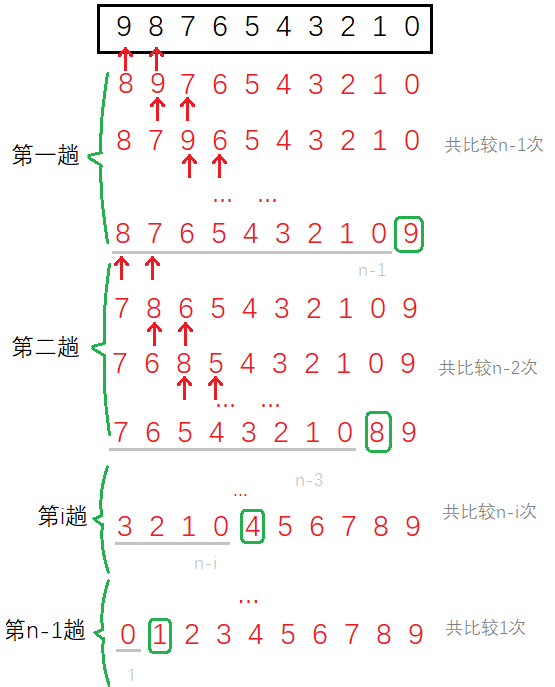
You can also look at the number of comparisons. Because the last time of each trip is only compared and not exchanged, the number of comparisons per trip is more than the number of exchanges. However, it does not affect its complexity.

Example 4

int BinarySearch(int* a, int n, int x) {
	assert(a);
	int begin = 0;
	int end = n - 1;
	while (begin < end) {
		int mid = begin + ((end - begin) >> 1);
		if (a[mid] < x)
			begin = mid + 1;
		else if (a[mid] > x)
			end = mid;
		else
			return mid;
	}
	return -1;
}

The complexity of the algorithm depends not only on the number of layers of the loop, but also on the idea of the algorithm. Binary search also has the best case and the worst case, and its worst case (not found) still needs to be analyzed.

For such a case, we can use the "origami method" to understand it vividly. A piece of paper is folded in half, removed in half, folded in half, and then discarded. It is assumed that there are a total of folds x x x times, the number is found. that is 2 x = N 2^x=N 2x=N, so the number of times x = l o g 2 N x=log_2N x=log2​N .

Logarithmic order O ( l o g 2 N ) O(log_2N) O(log2 ＾ N), or omit the base and write it as O ( l o g N ) O(logN) O(logN). The logarithmic order of binary search is a very excellent algorithm, 20 = l o g 2 ( 1000000 ) 20=log_2(1000000) 20=log2 (1000000), the number of one million only needs to be searched 20 times.

Example 5

long Factorial(size_t N)
{
	if (0 == N)
		return 1;
	return Fac(N - 1) * N;
}

The complexity of the recursive algorithm depends on two factors: the depth of recursion and the number of recursive calls per time.

Recursion depth is the total number of recursion layers, that is, the number of stack frames created. The number of recursive calls per time is the number of calls to itself within the recursive function.

Obviously, the depth of the problem is O ( N ) O(N) O(N), the number of calls is 1 1 1. Therefore, the complexity is O ( N ) O(N) O(N) .

Example 6

long Fibonacci(size_t N)
{
    if(N < 3)
        return 1;
    return Fib(N-1) + Fib(N-2);
}

Fibonacci's idea of recursion is similar to a binary tree, but there is a missing part, as shown in the figure:

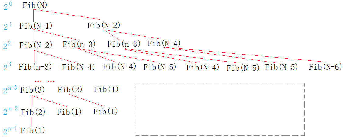
If there is no missing, it is a complete binary tree. Set the missing part as X X 10. The exact number of times is F ( N ) = 2 0 + 2 1 + 2 2 + . . . + 2 N − 1 − X = 2 N − 1 − X F(N)=2^0+2^1+2^2+...+2^{N-1}-X=2^N-1-X F(N)=20+21+22+...+2N − 1 − X=2N − 1 − X, because X X X is much less than 2 N − 1 2^N-1 2N − 1, so the complexity of the algorithm is O ( N ) = 2 N O(N)=2^N O(N)=2N.

 

Spatial complexity

Spatial complexity definition

Space complexity is also a mathematical expression, which measures the temporary additional storage space occupied by the algorithm when it runs. Similarly, the space complexity is not meaningless and the number of bytes actually occupied. The space complexity calculates the number of temporary variables. The basic rules are similar to the time complexity, and the large O asymptotic representation is also adopted.

Example 1

void BubbleSort(int* a, int n) {
	assert(a);
	for (size_t end = n; end > 0; --end) {
		int exchange = 0;
		for (size_t i = 1; i < end; ++i) {
			if (a[i - 1] > a[i]) {
				Swap(&a[i - 1], &a[i]);
				exchange = 1;
			}
		}
		if (exchange == 0)
			break;
	}
}

Bubble sorting algorithm only creates constant variables, so the spatial complexity is O ( 1 ) O(1) O(1).

Although the variables end and I are created once every cycle, in fact, from the perspective of memory, the space occupied each time will not change, and they are generally opened up in the same space.

Example 2

long long* Fibonacci(size_t n) {
    if (n == 0)
        return NULL;
    long long* fibArray = (long long*)malloc((n + 1) * sizeof(long long));
    fibArray[0] = 0;
    fibArray[1] = 1;
    for (int i = 2; i <= n; ++i) {
        fibArray[i] = fibArray[i - 1] + fibArray[i - 2];
    }
    return fibArray;
}

Including loop variables and the Fibonacci array, with the order of N N N variables. Therefore, the spatial complexity is O ( N ) O(N) O(N) .

Example 3

long long Factorial(size_t N)
{
    if(N == 0)
        return 1;
    return Fac(N - 1) * N;
}

Each time a stack frame is created recursively, there are constant variables in each stack frame, N N The space complexity of N-th recursion is O ( N ) O(N) O(N) .

The spatial complexity of recursion is related to the depth of recursion.

Example 4

long Fibonacci(size_t N)
{
    if(N < 3)
        return 1;
    return Fib(N-1) + Fib(N-2);
}

Fibonacci creates constant variables every time it recurses. As can be seen from the Fibonacci stack frame creation diagram, there will be duplicate items in the recursion, and these duplicate stack frames will be created and destroyed. Space is different from time and can be reused, so these repeated stack frames only occupy space once. therefore F i b ( N ) Fib(N) Fib(N), F i b ( N − 1 ) Fib(N-1) Fib(N−1),..., F i b ( 1 ) Fib(1) Fig (1) it is sufficient to allocate space once for these stack frames. Therefore, the time complexity is O ( N ) O(N) O(N) .

 

Common complexity

The complexity of common algorithms is shown in the following table. The complexity increases from top to bottom:

abbreviation	Large O indicates	Example
Constant order	O ( 1 ) O(1) O(1)	k k k
Logarithmic order	O ( l o g n ) O(logn) O(logn)	k l o g 2 n klog_2n klog2​n
Linear order	O ( n ) O(n) O(n)	k n kn kn
Logarithmic order	O ( n l o g n ) O(nlogn) O(nlogn)	k l o g 2 n klog_2n klog2​n
Square order	O ( n 2 ) O(n^2) O(n2)	k n 2 kn^2 kn2
Cubic order	O ( n 3 ) O(n^3) O(n3)	k n 3 kn^3 kn3
Exponential order	O ( 2 n ) O(2^n) O(2n)	k 2 n k2^n k2n
Factorial order	O ( n ! ) O(n!) O(n!)	k n ! kn! kn!

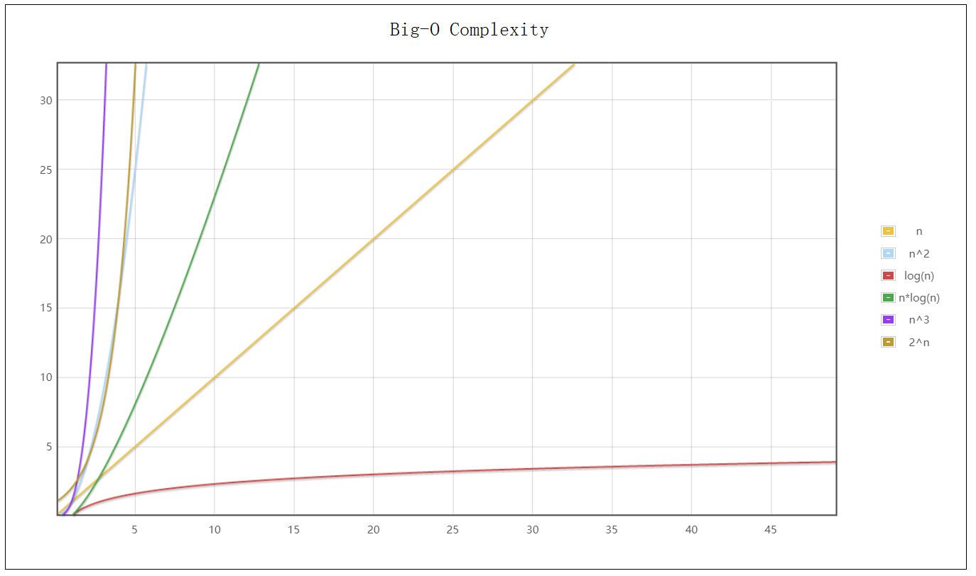
The lowest is constant times O ( 1 ) O(1) O(1), followed by logarithmic order O ( l o g n ) O(logn) O(logn), then linear order O ( n ) O(n) O(n), the higher is the square order O ( n 2 ) O(n^2) O(n2), the maximum is exponential order O ( 2 n ) O(2^n) O(2n) . The first three are excellent algorithms, while the square order is a complex algorithm. The algorithm of exponential order and factorial order is not advisable.

 

Complexity OJ problem

Disappearing numbers

Train of thought 1

First sort the array and check the difference between adjacent elements of the sorting result. If the difference is not 1, the missing value between them is the number that disappears.

The time complexity is O ( n l o g 2 n ) O(nlog_2n) O(nlog2# n), spatial complexity O ( 1 ) O(1) O(1)

int cmp_int(const void* e1, const void* e2) {
    return *(int*)e1 - *(int*)e2;
}
int missingNumber(int* nums, int numsSize) {
    qsort(nums, numsSize, sizeof(nums[0]), cmp_int);
    for(int i = 0; i < numsSize; i++) {
        if(nums[i +1] - nums[i] != 1) {
            return nums[i] + 1;
        }
    }
    return 0;
}

Train of thought 2

Write the elements in the array to the corresponding subscript position of another array. The subscript where there is no value is the missing number.

The time complexity is O ( n ) O(n) O(n), spatial complexity O ( n ) O(n) O(n)

int missingNumber(int* nums, int numsSize) {
    int tmp[200000] = { 0 };
    memset(tmp, -1, 200000 * sizeof(int));
    //Move in element
    for (int i = 0; i < numsSize; i++) {
        tmp[nums[i]] = nums[i];
    }
    //Find location
    for (int i = 0; i <= numsSize; i++) {
        if(tmp[i] == -1) {
            return i;
        }
    }
    return 0;
}

Train of thought 3

Subtract the sum of the elements from 0 to n from the sum of the array elements, and the result is the missing number.

The time complexity is O ( n ) O(n) O(n), spatial complexity O ( 1 ) O(1) O(1)

int missingNumber(int* nums, int numsSize) {
    int sumOfNum = 0;
    int sumOfNums = 0;
    for (int i = 0; i <= numsSize; i++) {
        sumOfNum += i;
    }
    for (int i = 0; i < numsSize; i++) {
        sumOfNums += nums[i];
    }
    return sumOfNum - sumOfNums;
}

Train of thought 4

take x x x and [ 0 , n ] [0,n] The number of [0,n] traverses XOR. When traversing XOR with array elements, the final result is the number that disappears.

The time complexity is O ( n ) O(n) O(n), spatial complexity O ( 1 ) O(1) O(1)

int missingNumber(int* nums, int numsSize) {
    int xor = 0;
    //And [0,n] XOR
    for (int i = 0; i <= numsSize; i++) {
        xor ^= i;
    }
    //And array XOR
    for (int i = 0; i < numsSize; i++) {
        xor ^= nums[i];
    }
    return xor;
}

Rotate array

Train of thought 1

Delete the tail of the array once, insert the tail element of the original array in the head, and loop k k k times.

The time complexity is O ( k × n ) O(k×n) O(k × n) , spatial complexity O ( 1 ) O(1) O(1)

void rotate(int* nums, int numsSize, int k) {
    while (k--) {
        int tmp = nums[numsSize - 1];
        int end = numsSize - 1;
        while (end > 0) {
            nums[end] = nums[end - 1] ;
            end--;
        }
        nums[end] = tmp;
    }
}

Train of thought 2

Open up an array of the same size, and then n − k n-k n − k elements are transferred to the past before the transfer k k k elements, in the return array.

The time complexity is O ( n ) O(n) O(n), spatial complexity O ( n ) O(n) O(n)

void rotate(int* nums, int numsSize, int k) {
    int tmp[200] = { 0 };
    //Last k
    for (int i = 0; i < k; i++) {
        tmp[i] = nums[numsSize - k + i];
    }
    //First k
    for (int i = 0; i < numsSize - k; i++) {
        tmp[i + k] = nums[i];
    }
    //transfer
    for (int i = 0; i < numsSize; i++) {
        nums[i] = tmp[i];
    }
}

Train of thought 3

front n − k n-k n − k elements are reversed, and then k k k elements are inverted, and then the whole is inverted.

The time complexity is O ( n ) O(n) O(n), spatial complexity O ( 1 ) O(1) O(1)

void reserve(int* nums, int left, int right) {
    while (left < right) {
        int tmp = nums[left];
        nums[left] = nums[right];
        nums[right] = tmp;
        left++;
        right--;
    }
}
void rotate(int* nums, int numsSize, int k) {
    //1. First n-k inversions
    reserve(nums, 0, numsSize -k - 1);
    //2. The last k inverses
    reserve(nums,numsSize - k, numsSize - 1);
    //3. Overall reverse
    reserve(nums, 0, numsSize - 1);
}