1. sklearn dataset
1.1 Dataset Partitioning
Machine learning general datasets are divided into two parts:
Training data: for training, building models
Test data: Used during model validation to assess whether a model is valid
SklearnDataset Partitioning API: sklearn.model_selection.train_test_split
1.2 Introduction to sklearn dataset interface
Introduction to the scikit-learn dataset API:
sklearn.datasets
- Load Get Popular Datasets
- datasets.load_*()
- Get small-scale datasets, data contained in datasets
- datasets.fetch_*(data_home=None)
- To get large datasets, you need to download them from the network. The first parameter to the function is data_home, which represents the dataset
- Downloaded directory, default is ~/scikit_learn_data/
Gets the type returned by the dataset:
Data type datasets.base.Bunch (dictionary format) returned by load*and fetch*
- Data: An array of characteristic data, which is a two-dimensional numpy.ndarray array of [n_samples * n_features]
- target: Tag array, which is a one-dimensional numpy.ndarray array of n_samples
- DESCR: Data Description
- feature_names: feature names, news data, handwritten numbers, regression datasets do not have
- target_names: Tag name, regression dataset does not have
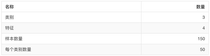
1.3 sklearn taxonomy dataset
sklearn.datasets.load_iris(): Load and return the Iris dataset.
sklearn.datasets.load_digits(): Loads and returns a digital dataset.

from sklearn.datasets import load_iris

li = load_iris()

print("Getting eigenvalues")
print(li.data)
print("target value")
print(li.target)
print(li.DESCR)
Run result:
Getting eigenvalues
[[5.1 3.5 1.4 0.2]
 [4.9 3.  1.4 0.2]
 [4.7 3.2 1.3 0.2]
 [4.6 3.1 1.5 0.2]
 [5.  3.6 1.4 0.2]
 [5.4 3.9 1.7 0.4]
 [4.6 3.4 1.4 0.3]
 [5.  3.4 1.5 0.2]
 [4.4 2.9 1.4 0.2]
 [4.9 3.1 1.5 0.1]
 [5.4 3.7 1.5 0.2]
 [4.8 3.4 1.6 0.2]
 [4.8 3.  1.4 0.1]
 [4.3 3.  1.1 0.1]
 [5.8 4.  1.2 0.2]
 [5.7 4.4 1.5 0.4]
 [5.4 3.9 1.3 0.4]
 [5.1 3.5 1.4 0.3]
 [5.7 3.8 1.7 0.3]
 [5.1 3.8 1.5 0.3]
 [5.4 3.4 1.7 0.2]
 [5.1 3.7 1.5 0.4]
 [4.6 3.6 1.  0.2]
 [5.1 3.3 1.7 0.5]
 [4.8 3.4 1.9 0.2]
 [5.  3.  1.6 0.2]
 [5.  3.4 1.6 0.4]
 [5.2 3.5 1.5 0.2]
 [5.2 3.4 1.4 0.2]
 [4.7 3.2 1.6 0.2]
 [4.8 3.1 1.6 0.2]
 [5.4 3.4 1.5 0.4]
 [5.2 4.1 1.5 0.1]
 [5.5 4.2 1.4 0.2]
 [4.9 3.1 1.5 0.2]
 [5.  3.2 1.2 0.2]
 [5.5 3.5 1.3 0.2]
 [4.9 3.6 1.4 0.1]
 [4.4 3.  1.3 0.2]
 [5.1 3.4 1.5 0.2]
 [5.  3.5 1.3 0.3]
 [4.5 2.3 1.3 0.3]
 [4.4 3.2 1.3 0.2]
 [5.  3.5 1.6 0.6]
 [5.1 3.8 1.9 0.4]
 [4.8 3.  1.4 0.3]
 [5.1 3.8 1.6 0.2]
 [4.6 3.2 1.4 0.2]
 [5.3 3.7 1.5 0.2]
 [5.  3.3 1.4 0.2]
 [7.  3.2 4.7 1.4]
 [6.4 3.2 4.5 1.5]
 [6.9 3.1 4.9 1.5]
 [5.5 2.3 4.  1.3]
 [6.5 2.8 4.6 1.5]
 [5.7 2.8 4.5 1.3]
 [6.3 3.3 4.7 1.6]
 [4.9 2.4 3.3 1. ]
 [6.6 2.9 4.6 1.3]
 [5.2 2.7 3.9 1.4]
 [5.  2.  3.5 1. ]
 [5.9 3.  4.2 1.5]
 [6.  2.2 4.  1. ]
 [6.1 2.9 4.7 1.4]
 [5.6 2.9 3.6 1.3]
 [6.7 3.1 4.4 1.4]
 [5.6 3.  4.5 1.5]
 [5.8 2.7 4.1 1. ]
 [6.2 2.2 4.5 1.5]
 [5.6 2.5 3.9 1.1]
 [5.9 3.2 4.8 1.8]
 [6.1 2.8 4.  1.3]
 [6.3 2.5 4.9 1.5]
 [6.1 2.8 4.7 1.2]
 [6.4 2.9 4.3 1.3]
 [6.6 3.  4.4 1.4]
 [6.8 2.8 4.8 1.4]
 [6.7 3.  5.  1.7]
 [6.  2.9 4.5 1.5]
 [5.7 2.6 3.5 1. ]
 [5.5 2.4 3.8 1.1]
 [5.5 2.4 3.7 1. ]
 [5.8 2.7 3.9 1.2]
 [6.  2.7 5.1 1.6]
 [5.4 3.  4.5 1.5]
 [6.  3.4 4.5 1.6]
 [6.7 3.1 4.7 1.5]
 [6.3 2.3 4.4 1.3]
 [5.6 3.  4.1 1.3]
 [5.5 2.5 4.  1.3]
 [5.5 2.6 4.4 1.2]
 [6.1 3.  4.6 1.4]
 [5.8 2.6 4.  1.2]
 [5.  2.3 3.3 1. ]
 [5.6 2.7 4.2 1.3]
 [5.7 3.  4.2 1.2]
 [5.7 2.9 4.2 1.3]
 [6.2 2.9 4.3 1.3]
 [5.1 2.5 3.  1.1]
 [5.7 2.8 4.1 1.3]
 [6.3 3.3 6.  2.5]
 [5.8 2.7 5.1 1.9]
 [7.1 3.  5.9 2.1]
 [6.3 2.9 5.6 1.8]
 [6.5 3.  5.8 2.2]
 [7.6 3.  6.6 2.1]
 [4.9 2.5 4.5 1.7]
 [7.3 2.9 6.3 1.8]
 [6.7 2.5 5.8 1.8]
 [7.2 3.6 6.1 2.5]
 [6.5 3.2 5.1 2. ]
 [6.4 2.7 5.3 1.9]
 [6.8 3.  5.5 2.1]
 [5.7 2.5 5.  2. ]
 [5.8 2.8 5.1 2.4]
 [6.4 3.2 5.3 2.3]
 [6.5 3.  5.5 1.8]
 [7.7 3.8 6.7 2.2]
 [7.7 2.6 6.9 2.3]
 [6.  2.2 5.  1.5]
 [6.9 3.2 5.7 2.3]
 [5.6 2.8 4.9 2. ]
 [7.7 2.8 6.7 2. ]
 [6.3 2.7 4.9 1.8]
 [6.7 3.3 5.7 2.1]
 [7.2 3.2 6.  1.8]
 [6.2 2.8 4.8 1.8]
 [6.1 3.  4.9 1.8]
 [6.4 2.8 5.6 2.1]
 [7.2 3.  5.8 1.6]
 [7.4 2.8 6.1 1.9]
 [7.9 3.8 6.4 2. ]
 [6.4 2.8 5.6 2.2]
 [6.3 2.8 5.1 1.5]
 [6.1 2.6 5.6 1.4]
 [7.7 3.  6.1 2.3]
 [6.3 3.4 5.6 2.4]
 [6.4 3.1 5.5 1.8]
 [6.  3.  4.8 1.8]
 [6.9 3.1 5.4 2.1]
 [6.7 3.1 5.6 2.4]
 [6.9 3.1 5.1 2.3]
 [5.8 2.7 5.1 1.9]
 [6.8 3.2 5.9 2.3]
 [6.7 3.3 5.7 2.5]
 [6.7 3.  5.2 2.3]
 [6.3 2.5 5.  1.9]
 [6.5 3.  5.2 2. ]
 [6.2 3.4 5.4 2.3]
 [5.9 3.  5.1 1.8]]
//target value
[0 0 0 0 0 0 0 0 0 0 0 0 0 0 0 0 0 0 0 0 0 0 0 0 0 0 0 0 0 0 0 0 0 0 0 0 0
 0 0 0 0 0 0 0 0 0 0 0 0 0 1 1 1 1 1 1 1 1 1 1 1 1 1 1 1 1 1 1 1 1 1 1 1 1
 1 1 1 1 1 1 1 1 1 1 1 1 1 1 1 1 1 1 1 1 1 1 1 1 1 1 2 2 2 2 2 2 2 2 2 2 2
 2 2 2 2 2 2 2 2 2 2 2 2 2 2 2 2 2 2 2 2 2 2 2 2 2 2 2 2 2 2 2 2 2 2 2 2 2
 2 2]
.. _iris_dataset:

Iris plants dataset
--------------------

**Data Set Characteristics:**

    :Number of Instances: 150 (50 in each of three classes)
    :Number of Attributes: 4 numeric, predictive attributes and the class
    :Attribute Information:
        - sepal length in cm
        - sepal width in cm
        - petal length in cm
        - petal width in cm
        - class:
                - Iris-Setosa
                - Iris-Versicolour
                - Iris-Virginica

    :Summary Statistics:

    ============== ==== ==== ======= ===== ====================
                    Min  Max   Mean    SD   Class Correlation
    ============== ==== ==== ======= ===== ====================
    sepal length:   4.3  7.9   5.84   0.83    0.7826
    sepal width:    2.0  4.4   3.05   0.43   -0.4194
    petal length:   1.0  6.9   3.76   1.76    0.9490  (high!)
    petal width:    0.1  2.5   1.20   0.76    0.9565  (high!)
    ============== ==== ==== ======= ===== ====================

    :Missing Attribute Values: None
    :Class Distribution: 33.3% for each of 3 classes.
    :Creator: R.A. Fisher
    :Donor: Michael Marshall (MARSHALL%PLU@io.arc.nasa.gov)
    :Date: July, 1988

The famous Iris database, first used by Sir R.A. Fisher. The dataset is taken
from Fisher's paper. Note that it's the same as in R, but not as in the UCI
Machine Learning Repository, which has two wrong data points.

This is perhaps the best known database to be found in the
pattern recognition literature.  Fisher's paper is a classic in the field and
is referenced frequently to this day.  (See Duda & Hart, for example.)  The
data set contains 3 classes of 50 instances each, where each class refers to a
type of iris plant.  One class is linearly separable from the other 2; the
latter are NOT linearly separable from each other.

.. topic:: References

   - Fisher, R.A. "The use of multiple measurements in taxonomic problems"
     Annual Eugenics, 7, Part II, 179-188 (1936); also in "Contributions to
     Mathematical Statistics" (John Wiley, NY, 1950).
   - Duda, R.O., & Hart, P.E. (1973) Pattern Classification and Scene Analysis.
     (Q327.D83) John Wiley & Sons.  ISBN 0-471-22361-1.  See page 218.
   - Dasarathy, B.V. (1980) "Nosing Around the Neighborhood: A New System
     Structure and Classification Rule for Recognition in Partially Exposed
     Environments".  IEEE Transactions on Pattern Analysis and Machine
     Intelligence, Vol. PAMI-2, No. 1, 67-71.
   - Gates, G.W. (1972) "The Reduced Nearest Neighbor Rule".  IEEE Transactions
     on Information Theory, May 1972, 431-433.
   - See also: 1988 MLC Proceedings, 54-64.  Cheeseman et al"s AUTOCLASS II
     conceptual clustering system finds 3 classes in the data.
   - Many, many more ...
1.4 Segmentation of datasets
sklearn.model_selection.train_test_split(*arrays, **options)
x: The characteristic value of the dataset
y: The label value of the dataset
test_size: The size of the test set, typically float
random_state: Random number seeds, different seeds will result in different random sampling results.Same seed sampling results are the same.
return: training set eigenvalues, test set eigenvalues, training labels, test labels (default random selection)
from sklearn.datasets import load_iris
from sklearn.model_selection import train_test_split

li = load_iris()

# Notice the return value, training set train  x_train, y_train        Test Set  test   x_test, y_test
x_train, x_test, y_train, y_test = train_test_split(li.data, li.target, test_size=0.25)

print("Training set eigenvalues and target values:", x_train, y_train)
print("Test set eigenvalues and target values:", x_test, y_test)
Run result:
Training set eigenvalues and target values: [[5.1 3.4 1.5 0.2]
 [6.7 3.1 4.4 1.4]
 [5.8 2.7 5.1 1.9]
 [5.2 3.5 1.5 0.2]
 [6.3 3.4 5.6 2.4]
 [5.9 3.  4.2 1.5]
 [5.6 2.7 4.2 1.3]
 [4.7 3.2 1.6 0.2]
 [6.5 2.8 4.6 1.5]
 [6.1 3.  4.6 1.4]
 [4.4 2.9 1.4 0.2]
 [5.8 2.7 5.1 1.9]
 [6.4 2.8 5.6 2.2]
 [7.6 3.  6.6 2.1]
 [6.6 3.  4.4 1.4]
 [4.6 3.2 1.4 0.2]
 [5.7 2.5 5.  2. ]
 [5.1 3.8 1.9 0.4]
 [6.7 3.3 5.7 2.1]
 [5.7 2.6 3.5 1. ]
 [5.1 3.5 1.4 0.3]
 [6.7 3.1 5.6 2.4]
 [5.6 3.  4.1 1.3]
 [5.5 3.5 1.3 0.2]
 [4.6 3.6 1.  0.2]
 [5.7 3.8 1.7 0.3]
 [6.  3.  4.8 1.8]
 [6.2 2.9 4.3 1.3]
 [7.3 2.9 6.3 1.8]
 [5.  3.  1.6 0.2]
 [4.8 3.1 1.6 0.2]
 [6.3 2.5 5.  1.9]
 [5.5 2.6 4.4 1.2]
 [5.1 3.3 1.7 0.5]
 [6.6 2.9 4.6 1.3]
 [4.8 3.  1.4 0.3]
 [5.4 3.9 1.3 0.4]
 [6.7 3.  5.2 2.3]
 [4.8 3.4 1.6 0.2]
 [7.1 3.  5.9 2.1]
 [6.9 3.1 4.9 1.5]
 [6.4 3.1 5.5 1.8]
 [5.  3.4 1.6 0.4]
 [6.  2.7 5.1 1.6]
 [6.3 2.8 5.1 1.5]
 [5.7 4.4 1.5 0.4]
 [6.3 2.9 5.6 1.8]
 [5.  3.2 1.2 0.2]
 [6.  3.4 4.5 1.6]
 [6.3 2.7 4.9 1.8]
 [4.9 3.1 1.5 0.1]
 [5.8 2.7 4.1 1. ]
 [5.4 3.7 1.5 0.2]
 [7.2 3.  5.8 1.6]
 [5.1 3.7 1.5 0.4]
 [6.3 2.5 4.9 1.5]
 [4.4 3.2 1.3 0.2]
 [6.4 2.8 5.6 2.1]
 [4.6 3.4 1.4 0.3]
 [5.4 3.9 1.7 0.4]
 [6.  2.9 4.5 1.5]
 [6.8 2.8 4.8 1.4]
 [5.9 3.2 4.8 1.8]
 [5.1 2.5 3.  1.1]
 [6.9 3.1 5.1 2.3]
 [7.9 3.8 6.4 2. ]
 [4.4 3.  1.3 0.2]
 [6.9 3.1 5.4 2.1]
 [5.7 2.9 4.2 1.3]
 [5.4 3.  4.5 1.5]
 [6.8 3.  5.5 2.1]
 [6.7 3.1 4.7 1.5]
 [4.9 2.4 3.3 1. ]
 [5.2 4.1 1.5 0.1]
 [6.5 3.  5.5 1.8]
 [6.  2.2 4.  1. ]
 [5.3 3.7 1.5 0.2]
 [4.3 3.  1.1 0.1]
 [5.6 3.  4.5 1.5]
 [6.  2.2 5.  1.5]
 [4.7 3.2 1.3 0.2]
 [6.2 2.2 4.5 1.5]
 [5.6 2.5 3.9 1.1]
 [5.  3.5 1.6 0.6]
 [5.5 2.3 4.  1.3]
 [5.2 2.7 3.9 1.4]
 [6.4 2.9 4.3 1.3]
 [5.2 3.4 1.4 0.2]
 [5.1 3.8 1.5 0.3]
 [6.7 2.5 5.8 1.8]
 [5.1 3.8 1.6 0.2]
 [7.2 3.2 6.  1.8]
 [5.7 2.8 4.1 1.3]
 [6.7 3.  5.  1.7]
 [6.2 3.4 5.4 2.3]
 [6.9 3.2 5.7 2.3]
 [6.1 3.  4.9 1.8]
 [4.9 2.5 4.5 1.7]
 [5.8 2.6 4.  1.2]
 [4.8 3.4 1.9 0.2]
 [5.6 2.9 3.6 1.3]
 [4.5 2.3 1.3 0.3]
 [6.1 2.8 4.  1.3]
 [7.7 2.8 6.7 2. ]
 [6.5 3.  5.2 2. ]
 [4.9 3.6 1.4 0.1]
 [6.1 2.8 4.7 1.2]
 [5.  3.5 1.3 0.3]
 [6.8 3.2 5.9 2.3]
 [5.  3.3 1.4 0.2]
 [5.7 2.8 4.5 1.3]
 [4.9 3.  1.4 0.2]] [0 1 2 0 2 1 1 0 1 1 0 2 2 2 1 0 2 0 2 1 0 2 1 0 0 0 2 1 2 0 0 2 1 0 1 0 0
 2 0 2 1 2 0 1 2 0 2 0 1 2 0 1 0 2 0 1 0 2 0 0 1 1 1 1 2 2 0 2 1 1 2 1 1 0
 2 1 0 0 1 2 0 1 1 0 1 1 1 0 0 2 0 2 1 1 2 2 2 2 1 0 1 0 1 2 2 0 1 0 2 0 1
 0]
Test set eigenvalues and target values: [[7.7 2.6 6.9 2.3]
 [6.4 3.2 5.3 2.3]
 [5.5 2.5 4.  1.3]
 [5.1 3.5 1.4 0.2]
 [5.7 3.  4.2 1.2]
 [5.  3.4 1.5 0.2]
 [7.2 3.6 6.1 2.5]
 [5.5 2.4 3.7 1. ]
 [5.  2.  3.5 1. ]
 [5.9 3.  5.1 1.8]
 [6.5 3.  5.8 2.2]
 [5.  2.3 3.3 1. ]
 [4.8 3.  1.4 0.1]
 [4.9 3.1 1.5 0.2]
 [5.5 2.4 3.8 1.1]
 [7.7 3.  6.1 2.3]
 [5.8 2.8 5.1 2.4]
 [6.7 3.3 5.7 2.5]
 [7.7 3.8 6.7 2.2]
 [7.4 2.8 6.1 1.9]
 [5.8 4.  1.2 0.2]
 [6.1 2.6 5.6 1.4]
 [6.3 3.3 6.  2.5]
 [6.4 2.7 5.3 1.9]
 [5.5 4.2 1.4 0.2]
 [5.8 2.7 3.9 1.2]
 [6.1 2.9 4.7 1.4]
 [4.6 3.1 1.5 0.2]
 [5.6 2.8 4.9 2. ]
 [6.3 2.3 4.4 1.3]
 [5.4 3.4 1.7 0.2]
 [5.4 3.4 1.5 0.4]
 [5.  3.6 1.4 0.2]
 [6.2 2.8 4.8 1.8]
 [7.  3.2 4.7 1.4]
 [6.4 3.2 4.5 1.5]
 [6.5 3.2 5.1 2. ]
 [6.3 3.3 4.7 1.6]] [2 2 1 0 1 0 2 1 1 2 2 1 0 0 1 2 2 2 2 2 0 2 2 2 0 1 1 0 2 1 0 0 0 2 1 1 2
 1]
1.5 Large datasets for classification
sklearn.datasets.fetch_20newsgroups(data_home=None,subset='train')
Subset:'train'or'test','all', optional, select the dataset to load.
"Training" of the training set and "Test" of the test set, both "All"
datasets.clear_data_home(data_home=None): Clear data from directory
from sklearn.datasets import fetch_20newsgroups

news = fetch_20newsgroups(subset='all')

print(news.data)
print(news.target)
The first run downloads files, takes a long time, and the download data is huge.

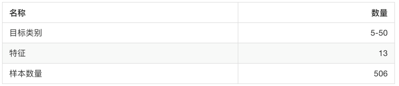
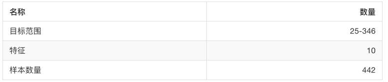
1.6 sklearn Regression Dataset
sklearn.datasets.load_boston(): Load and return the Boston housing price data set.
sklearn.datasets.load_diabetes(): Load and return the diabetes dataset.
from sklearn.datasets import load_boston

lb = load_boston()

print("Getting eigenvalues")
print(lb.data)
print("target value")
print(lb.target)
print(lb.DESCR)
Run result:
Getting eigenvalues
[[6.3200e-03 1.8000e+01 2.3100e+00 ... 1.5300e+01 3.9690e+02 4.9800e+00]
 [2.7310e-02 0.0000e+00 7.0700e+00 ... 1.7800e+01 3.9690e+02 9.1400e+00]
 [2.7290e-02 0.0000e+00 7.0700e+00 ... 1.7800e+01 3.9283e+02 4.0300e+00]
 ...
 [6.0760e-02 0.0000e+00 1.1930e+01 ... 2.1000e+01 3.9690e+02 5.6400e+00]
 [1.0959e-01 0.0000e+00 1.1930e+01 ... 2.1000e+01 3.9345e+02 6.4800e+00]
 [4.7410e-02 0.0000e+00 1.1930e+01 ... 2.1000e+01 3.9690e+02 7.8800e+00]]
//target value
[24.  21.6 34.7 33.4 36.2 28.7 22.9 27.1 16.5 18.9 15.  18.9 21.7 20.4
 18.2 19.9 23.1 17.5 20.2 18.2 13.6 19.6 15.2 14.5 15.6 13.9 16.6 14.8
 18.4 21.  12.7 14.5 13.2 13.1 13.5 18.9 20.  21.  24.7 30.8 34.9 26.6
 25.3 24.7 21.2 19.3 20.  16.6 14.4 19.4 19.7 20.5 25.  23.4 18.9 35.4
 24.7 31.6 23.3 19.6 18.7 16.  22.2 25.  33.  23.5 19.4 22.  17.4 20.9
 24.2 21.7 22.8 23.4 24.1 21.4 20.  20.8 21.2 20.3 28.  23.9 24.8 22.9
 23.9 26.6 22.5 22.2 23.6 28.7 22.6 22.  22.9 25.  20.6 28.4 21.4 38.7
 43.8 33.2 27.5 26.5 18.6 19.3 20.1 19.5 19.5 20.4 19.8 19.4 21.7 22.8
 18.8 18.7 18.5 18.3 21.2 19.2 20.4 19.3 22.  20.3 20.5 17.3 18.8 21.4
 15.7 16.2 18.  14.3 19.2 19.6 23.  18.4 15.6 18.1 17.4 17.1 13.3 17.8
 14.  14.4 13.4 15.6 11.8 13.8 15.6 14.6 17.8 15.4 21.5 19.6 15.3 19.4
 17.  15.6 13.1 41.3 24.3 23.3 27.  50.  50.  50.  22.7 25.  50.  23.8
 23.8 22.3 17.4 19.1 23.1 23.6 22.6 29.4 23.2 24.6 29.9 37.2 39.8 36.2
 37.9 32.5 26.4 29.6 50.  32.  29.8 34.9 37.  30.5 36.4 31.1 29.1 50.
 33.3 30.3 34.6 34.9 32.9 24.1 42.3 48.5 50.  22.6 24.4 22.5 24.4 20.
 21.7 19.3 22.4 28.1 23.7 25.  23.3 28.7 21.5 23.  26.7 21.7 27.5 30.1
 44.8 50.  37.6 31.6 46.7 31.5 24.3 31.7 41.7 48.3 29.  24.  25.1 31.5
 23.7 23.3 22.  20.1 22.2 23.7 17.6 18.5 24.3 20.5 24.5 26.2 24.4 24.8
 29.6 42.8 21.9 20.9 44.  50.  36.  30.1 33.8 43.1 48.8 31.  36.5 22.8
 30.7 50.  43.5 20.7 21.1 25.2 24.4 35.2 32.4 32.  33.2 33.1 29.1 35.1
 45.4 35.4 46.  50.  32.2 22.  20.1 23.2 22.3 24.8 28.5 37.3 27.9 23.9
 21.7 28.6 27.1 20.3 22.5 29.  24.8 22.  26.4 33.1 36.1 28.4 33.4 28.2
 22.8 20.3 16.1 22.1 19.4 21.6 23.8 16.2 17.8 19.8 23.1 21.  23.8 23.1
 20.4 18.5 25.  24.6 23.  22.2 19.3 22.6 19.8 17.1 19.4 22.2 20.7 21.1
 19.5 18.5 20.6 19.  18.7 32.7 16.5 23.9 31.2 17.5 17.2 23.1 24.5 26.6
 22.9 24.1 18.6 30.1 18.2 20.6 17.8 21.7 22.7 22.6 25.  19.9 20.8 16.8
 21.9 27.5 21.9 23.1 50.  50.  50.  50.  50.  13.8 13.8 15.  13.9 13.3
 13.1 10.2 10.4 10.9 11.3 12.3  8.8  7.2 10.5  7.4 10.2 11.5 15.1 23.2
  9.7 13.8 12.7 13.1 12.5  8.5  5.   6.3  5.6  7.2 12.1  8.3  8.5  5.
 11.9 27.9 17.2 27.5 15.  17.2 17.9 16.3  7.   7.2  7.5 10.4  8.8  8.4
 16.7 14.2 20.8 13.4 11.7  8.3 10.2 10.9 11.   9.5 14.5 14.1 16.1 14.3
 11.7 13.4  9.6  8.7  8.4 12.8 10.5 17.1 18.4 15.4 10.8 11.8 14.9 12.6
 14.1 13.  13.4 15.2 16.1 17.8 14.9 14.1 12.7 13.5 14.9 20.  16.4 17.7
 19.5 20.2 21.4 19.9 19.  19.1 19.1 20.1 19.9 19.6 23.2 29.8 13.8 13.3
 16.7 12.  14.6 21.4 23.  23.7 25.  21.8 20.6 21.2 19.1 20.6 15.2  7.
  8.1 13.6 20.1 21.8 24.5 23.1 19.7 18.3 21.2 17.5 16.8 22.4 20.6 23.9
 22.  11.9]
.. _boston_dataset:

Boston house prices dataset
---------------------------

**Data Set Characteristics:**

    :Number of Instances: 506

    :Number of Attributes: 13 numeric/categorical predictive. Median Value (attribute 14) is usually the target.

    :Attribute Information (in order):
        - CRIM     per capita crime rate by town
        - ZN       proportion of residential land zoned for lots over 25,000 sq.ft.
        - INDUS    proportion of non-retail business acres per town
        - CHAS     Charles River dummy variable (= 1 if tract bounds river; 0 otherwise)
        - NOX      nitric oxides concentration (parts per 10 million)
        - RM       average number of rooms per dwelling
        - AGE      proportion of owner-occupied units built prior to 1940
        - DIS      weighted distances to five Boston employment centres
        - RAD      index of accessibility to radial highways
        - TAX      full-value property-tax rate per $10,000
        - PTRATIO  pupil-teacher ratio by town
        - B        1000(Bk - 0.63)^2 where Bk is the proportion of blacks by town
        - LSTAT    % lower status of the population
        - MEDV     Median value of owner-occupied homes in $1000's

    :Missing Attribute Values: None

    :Creator: Harrison, D. and Rubinfeld, D.L.

This is a copy of UCI ML housing dataset.
https://archive.ics.uci.edu/ml/machine-learning-databases/housing/


This dataset was taken from the StatLib library which is maintained at Carnegie Mellon University.

The Boston house-price data of Harrison, D. and Rubinfeld, D.L. 'Hedonic
prices and the demand for clean air', J. Environ. Economics & Management,
vol.5, 81-102, 1978.   Used in Belsley, Kuh & Welsch, 'Regression diagnostics
...', Wiley, 1980.   N.B. Various transformations are used in the table on
pages 244-261 of the latter.

The Boston house-price data has been used in many machine learning papers that address regression
problems.

.. topic:: References

   - Belsley, Kuh & Welsch, 'Regression diagnostics: Identifying Influential Data and Sources of Collinearity', Wiley, 1980. 244-261.
   - Quinlan,R. (1993). Combining Instance-Based and Model-Based Learning. In Proceedings on the Tenth International Conference of Machine Learning, 236-243, University of Massachusetts, Amherst. Morgan Kaufmann.
1.7 Converter
How many steps did we take for feature engineering?
1. Instantiate (instantiating is a transformer class).
2. Call fit_transform() to establish a categorical word frequency matrix for a document, which cannot be called at the same time.
fit_transform(): Direct conversion of input data.
The fit_transform() method is actually a combination of fit() and transform() methods.
fit(): Enter data, but do nothing.
transform(): Convert data.
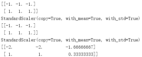
from  sklearn.preprocessing import StandardScaler

s = StandardScaler()
print(s.fit_transform([[1,2,3],[4,5,6]]))

ss = StandardScaler()
print(ss.fit([[1,2,3],[4,5,6]]))
print(ss.transform([[1,2,3],[4,5,6]]))
print(ss.fit([[2,3,4],[4,5,7]]))
print(ss.transform([[1,2,3],[4,5,6]]))
Run result:
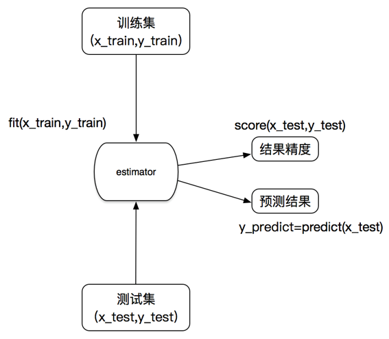
1.8 Estimator
In sklearn, estimator is an important role, classifier and regressor belong to estimator, which is a kind of API that implements algorithm
1. Estimators for classification:
sklearn.neighbors k-nearest neighbor algorithm
sklearn.naive_bayes Bayes
Sklearn.linear_model.Logistic Regression Logistic Regression
2. Estimators for regression:
sklearn.linear_model.LinearRegression linear regression
sklearn.linear_model.Ridge ridge regression
Estimator workflow: