Introduction of BP network prediction algorithm

1. Introduction to Artificial Neural Network

Artificial Neural Network (ANN) is a computer system formed by several very simple processing units connected to each other in some way to mimic the structure and function of the human brain. It processes information by the dynamic response of its state to the external input information.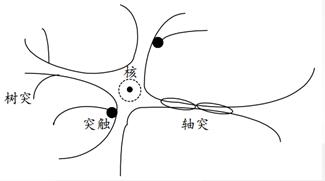

Neurons are composed of cells and many of the processes they emit. In cells, there are nuclei, and synapses act to transmit information. Several processes that act as input signals are called dendrites, while only one process that acts as output signals is called axons.

2. Neuronal M-P Model

The so-called M-P model is actually an abstract and simplified model constructed according to the structure and working principle of biological neurons.

For the j j j neuron, the input signal x I x_i x I is received from several other neurons. The synaptic strength is expressed as the real coefficient w I J w_{i j}w I j, which is the weighted value of the action of the I I I neuron on the J J neuron.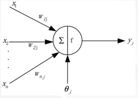

The net input of a neuron is expressed in I j I_jIj, which is a linear weighted sum, i.e.

The output y J y_j y J of the neuron j j is a function of its current state. The mathematical expression of the M-P model is:
[External chain picture transfer failed, source station may have anti-theft chain mechanism, it is recommended to save the picture and upload it directly (img-apKne9an-1615981917750). (https://img-blog.csdn.net/20170409215520699?watermark/2/text/aHR0cDovL2Jsb2cuY3Nkbi5uZXQvdTAxMDg1ODYwNQ==/font/5a6L5L2T/fontsize/400/fill/I0JBQkFCMA==/dissolve/70/gravity/SouthEast)]
In the formula, theta jtheta_jtheta J is the threshold value and s g n s g n s g n is the symbol function. When the net input exceeds the threshold value, y J y_j y J takes the + 1 output and vice versa is the -1 output. If the delay between output and input is considered, the expression can be modified to:

3. Basic elements of ANN

• Neuron activation function
• Learning on the Web
• Connection Forms Between Neurons

(1) Common activation functions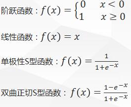

(2) Common learning rules

• Hebb Rule
• Error Correction Learning Algorithms (e.g., BP algorithm)
• Winner-Take-All learning rules

(3) Connection modes between neurons
<1>Prefix network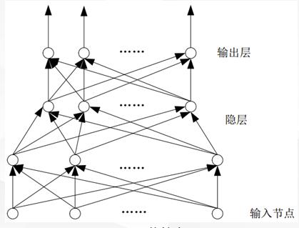

<2>Feedback Network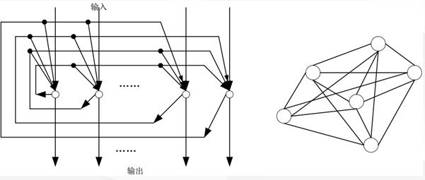

>Note: BP network belongs to prefix network

2. Principle of BP Network

BP (Back Propagation)The learning process of a neural network consists of two processes, the forward propagation of signals and the reverse propagation of errors. When the forward propagation occurs, input samples are passed in from the input layer and processed layer by layer, then transferred to the output layer. If the actual output of the output layer does not match the expected output, the reverse propagation of errors turns to the reverse propagation of errors. The reverse propagation of errors takes the output errors through the hidden layer in some form.BP network consists of input layer, output layer and hidden layer, N 1 N_1N 1 is input layer, N m N_mNm is output layer, and the rest is hidden layer. The structure of BP network is as follows: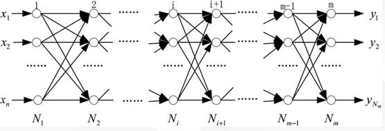

This paper introduces the derivation of a three-layer neural network (one input layer, one hidden layer and one output layer)

Neuron Schematic Diagram 1 of BP Neural Network Back Propagation Algorithm:

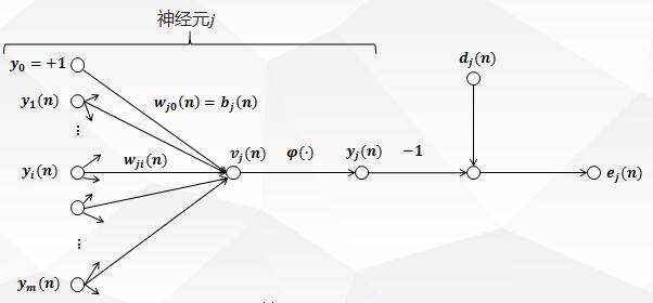
The figure above depicts the neuron j j fed to it by a set of functional signals produced by a layer of neurons on its left. m m m is the number of inputs that act on the neuron J J j, excluding offsets. The synaptic weight W J 0 (n) w_{j0} (n) w J0 (n) equals the offset B J b_j B J of the neuron J.

1. Derivation of forward propagation process

In Fig. 1, the induced local domain V J (n) v_j (n) v_j (n) V J (n) (i.e., the input of neuron J j) is generated at the input of the activation function of neuron J j:

The j \phi_j J is the activation function, and the function signal that appears at the output of the neuron j j j j (i.e. the output of the neuron J j) y J (n) y_j (n) y J (n) is:

2. Deduction of Error Back Propagation Process

In Fig. 1, y J (n) y_j (n) y J (n) and D J (n) d_j (n) D J (n) are the actual and expected output of neuron J j, respectively. The error signal produced by the output of neuron j j is defined as:

Where D J (n) d_j (n) D J (n) is the j j element of the expected response vector D (n) D (n) D (n).

In order to make the function continuously derivable, here the root mean square difference is minimized, and the instantaneous error energy of neuron j j is defined as:

Add the error energy of all output layer neurons to get the total instantaneous error energy of the whole network:

Set C contains all the neurons in the output layer.

BP BP algorithm minimizes E n E_nEn by iteratively modifying weights to minimize (2-5)E n E_nEn, and uses gradient descent to apply a modification to synaptic weights w J I (n) w_{j i}(n) W J I (n) using a gradient descent method using a modified value W J I (n) w {u{{j i}(n) 8710w {{j i}(n) \{j i}(n) \deltadeldeldelE ((n) / E(n) /E(n) /deldeldelta\\\\w_{j i}(n)w J i(n). According to the differential chain rule, this gradient is expressed as:

Partial derivative Delta Delta Delta Delta E (n) / E(n) / E(n) / E(n) / delta delta delta W J I (n) {j i} (n) W J I (n) represents a sensitive factor and determines the search direction of synaptic weight W J I w {j i} W J i i n the weight space.

Differentiating E J (n) e_j (n) e_j (n) E J (n) on both sides of equation (2-5) yields:

Differentiating y J (n) y_j (n) y_j (n) y J (n) on both sides of equation (2-3) yields:

Differentiating V J (n) v_j (n) v_j (n) V J (n) on both sides of equation (2-2) yields:

Finally, the W J I (n) w_{j i} (n) W J I (n) is differentiated on both sides of the formula (2-1) to get:

Put-in (2-7) - (2-10) get:

The modification W J I (n) w {j i} (n) W J I (n) applied to W J I (n) w {j i} (n) W J I (n) is defined as:

Among them, __eta is the learning rate of error reverse propagation, and a negative sign indicates that the gradient decreases in the weighted space.

The carry-in (2-11) form (2-12) is:

Where delta J \delta_j(n)delta j(n) is a local gradient defined by the delta rule:

Local gradients indicate the changes required for synaptic weights.

Now consider the layer where neuron j j j is located.

#####(1) Neuron j j j is the output layer node
When neuron j j is in the output layer, it is provided with an expected response. The local gradient delta J (n) delta_j (n) of neuron J is determined from the error signal E J (n) = D J (n) y J (n) = d_j (n) = d_j (n) -y_j (n) E J (n) = D J (n) y J (n) of equation (2-14). The local gradient delta_j (n) of neuron J is:

#####(2) Neuron j j j is a hidden node
There is no expected response to the input neuron when the neuron j j is in the recessive layer. The error signal of the recessive layer is determined recursively and backwards from the error signal of all the neurons directly connected to the recessive layer neuron.
Considering that the neuron J is a hidden layer node, the local gradient of the hidden layer neuron delta J \delta_j(n)delta j(n) is redefined as:

Consider Figure 2: It represents a signal flow diagram where the output layer neuron k k k connects to the hidden layer neuron J J.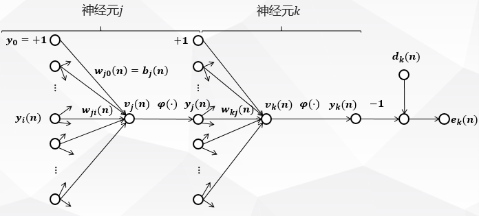

Here, the subscript j j j denotes the hidden layer neurons, and the subscript k k k denotes the output layer neurons.

In Figure 2, the total instantaneous error energy of the network is:

The derivative of the function signal Y J (n) y_j (n) y_j (n) y J (n) on both sides of formula (2-17) is obtained:

In Figure 2:

Therefore,

In Fig. 2, for the output layer neuron K K k, the induced local domain is:

The equation (2-21) derives the differentiation of Y J (n) y_j (n) y J (n):

Bring the formulas (2-20) and (2-22) into the formulas (2-18) to get:

The local gradient delta J (n) \delta_j(n) delta_j(n) Delta j(n) of the hidden layer neuron j j j is derived from the bring-in formula (2-16):

Derivation Summary of Reverse Propagation Process

Thus, the modified values of synaptic weights w J I (n) w {j i} (n) W J I (n) connected by neuron I I I to neuron j j i n conjunction with (2-13), (2-15) and (2-24) are defined as follows according to the delta rule:

Where:

• When the neuroneuron j j j j is the output layer node, the local gradient delj (n) \delta_j(n) delta_j(n) delta_j (delta_j(n) deldelj (delta_j(n) delj (n) delj (n) is equal to the reciprocal \j 'phi_j' \phi phi_j '(v_j (j (n) (v_j (n)) \j ((j j j j j j j j j j j j j j j j j j j j j j j j j) and the error signal E J (n) = D J (n) 8722;y J (e_j (n) =product of (n)y J (n), see formula (2-15);
• When neuron j j j is a hidden layer node, the local gradient delta J (n) delta_j(n) delta_j(n) delj(n) is equal to the product of the inverse j'(v J (n))phi_j' (v_j (n))j'(v J (n)) and the weighted sum of the delta_k delta K and the next layer (hidden or output layer), as shown in formula 2-24.

3. Design principles of standard BP network

(1) Activation function
Unipolar S-type function and hyperbolic tangent S-type function
(2) Learning rate
0 < η < 1 0<\eta<10<η<1
(3) Stop criteria
The mean square error of the network is small enough or the number of times it is trained is large enough, etc.
(4) Initial weight
Randomly select synaptic weights with uniform distribution of mean equal to 0
(5) Hidden layer structure
It is theoretically proved that one hidden layer can map all continuous functions.
Number of Hidden Layer Nodes = (Number of Input Nodes + Number of Output Nodes) \sqrt{(Number of Input Nodes + Number of Output Nodes)} (Number of Input Nodes + Number of Output Nodes) +alphaalpha, 1 <alpha<10 1<\alpha<101<alpha<10 or

Number of Hidden Layer Nodes = (Number of Input Nodes Number of Output Nodes) \sqrt{(Number of Input Nodes * Number of Output Nodes)} (Number of Input Nodes Number of Output Nodes)

4. Standard BP algorithm training process and flowchart

(1) Training process

1. Initialize the synaptic weights and threshold matrix of the network;

2. Presentation of training samples;

3. Forward propagation calculation;

4. Error back propagation calculates and updates weights;

5. Iterate through steps 3 and 4 with the new sample until the stop criteria are met.

(2) Flowchart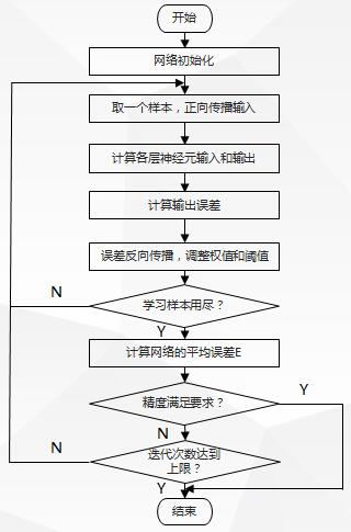

5. Analysis of Standard BP Algorithms

Since the standard BP algorithm uses the gradient descent method, the E-w curve of the BP algorithm is as follows: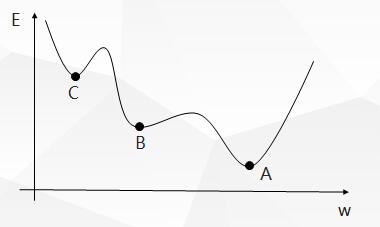

Therefore, the standard BP algorithm has the following drawbacks:

1. Some areas on the error surface are flat, at which time the error is not sensitive to the change of the weight value, the error decreases slowly, the adjustment time is long, and the convergence rate is affected.
2. There are many minimum points, so the gradient descent method is easy to fall into the minimum point and can not get the global optimal solution.
3. The smaller the learning rate_eta_is, the slower the learning speed will be, while the larger the learning speed will be, although the learning speed will be faster, it will be easy to make the change of weight unstable and oscillate.

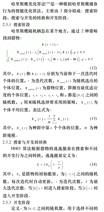
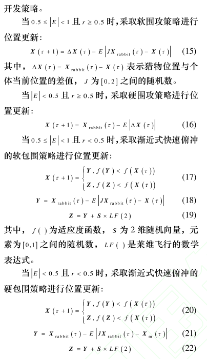
3. Harris Eagle algorithm

 

IV. Partial Codes

function [TrainingTime, TestingTime, TrainingAccuracy, TestingAccuracy] = elm_kernel(TrainingData, TestingData, Elm_Type, Regularization_coefficient, Kernel_type, Kernel_para)

% Usage: elm(TrainingData_File, TestingData_File, Elm_Type, NumberofHiddenNeurons, ActivationFunction)
% OR:    [TrainingTime, TestingTime, TrainingAccuracy, TestingAccuracy] = elm(TrainingData_File, TestingData_File, Elm_Type, NumberofHiddenNeurons, ActivationFunction)
%
% Input:
% TrainingData_File           - Filename of training data set

tic;
Omega_test = kernel_matrix(P',Kernel_type, Kernel_para,TV.P');
TY=(Omega_test' * OutputWeight)';                            %   TY: the actual output of the testing data
TestingTime=toc

%%%%%%%%%% Calculate training & testing classification accuracy

if Elm_Type == REGRESSION
%%%%%%%%%% Calculate training & testing accuracy (RMSE) for regression case
    TrainingAccuracy=sqrt(mse(T - Y))
    TestingAccuracy=sqrt(mse(TV.T - TY))           
end

if Elm_Type == CLASSIFIER
%%%%%%%%%% Calculate training & testing classification accuracy
    MissClassificationRate_Training=0;
    MissClassificationRate_Testing=0;

    for i = 1 : size(T, 2)
        [x, label_index_expected]=max(T(:,i));
        [x, label_index_actual]=max(Y(:,i));
        if label_index_actual~=label_index_expected
            MissClassificationRate_Training=MissClassificationRate_Training+1;
        end
    end
    TrainingAccuracy=1-MissClassificationRate_Training/size(T,2)  
    for i = 1 : size(TV.T, 2)
        [x, label_index_expected]=max(TV.T(:,i));
        [x, label_index_actual]=max(TY(:,i));
        if label_index_actual~=label_index_expected
            MissClassificationRate_Testing=MissClassificationRate_Testing+1;
        end
    end
    TestingAccuracy=(1-MissClassificationRate_Testing/size(TV.T,2))*100
end
    
    
%%%%%%%%%%%%%%%%%% Kernel Matrix %%%%%%%%%%%%%%%%%%%%%%%%%%%%%%%%%%%%%%%%%
    
function omega = kernel_matrix(Xtrain,kernel_type, kernel_pars,Xt)

nb_data = size(Xtrain,1);


if strcmp(kernel_type,'RBF_kernel'),
    if nargin<4,
        XXh = sum(Xtrain.^2,2)*ones(1,nb_data);
        omega = XXh+XXh'-2*(Xtrain*Xtrain');
        omega = exp(-omega./kernel_pars(1));
    else
        XXh1 = sum(Xtrain.^2,2)*ones(1,size(Xt,1));
        XXh2 = sum(Xt.^2,2)*ones(1,nb_data);
        omega = XXh1+XXh2' - 2*Xtrain*Xt';
        omega = exp(-omega./kernel_pars(1));
    end
    
elseif strcmp(kernel_type,'lin_kernel')
    if nargin<4,
        omega = Xtrain*Xtrain';
    else
        omega = Xtrain*Xt';
    end
    
elseif strcmp(kernel_type,'poly_kernel')
    if nargin<4,
        omega = (Xtrain*Xtrain'+kernel_pars(1)).^kernel_pars(2);
    else
        omega = (Xtrain*Xt'+kernel_pars(1)).^kernel_pars(2);
    end
    
elseif strcmp(kernel_type,'wav_kernel')
    if nargin<4,
        XXh = sum(Xtrain.^2,2)*ones(1,nb_data);
        omega = XXh+XXh'-2*(Xtrain*Xtrain');
        
        XXh1 = sum(Xtrain,2)*ones(1,nb_data);
        omega1 = XXh1-XXh1';
        omega = cos(kernel_pars(3)*omega1./kernel_pars(2)).*exp(-omega./kernel_pars(1));
        
    else
        XXh1 = sum(Xtrain.^2,2)*ones(1,size(Xt,1));
        XXh2 = sum(Xt.^2,2)*ones(1,nb_data);
        omega = XXh1+XXh2' - 2*(Xtrain*Xt');
        
        XXh11 = sum(Xtrain,2)*ones(1,size(Xt,1));
        XXh22 = sum(Xt,2)*ones(1,nb_data);
        omega1 = XXh11-XXh22';
        
        omega = cos(kernel_pars(3)*omega1./kernel_pars(2)).*exp(-omega./kernel_pars(1));
    end
end

5. Simulation results

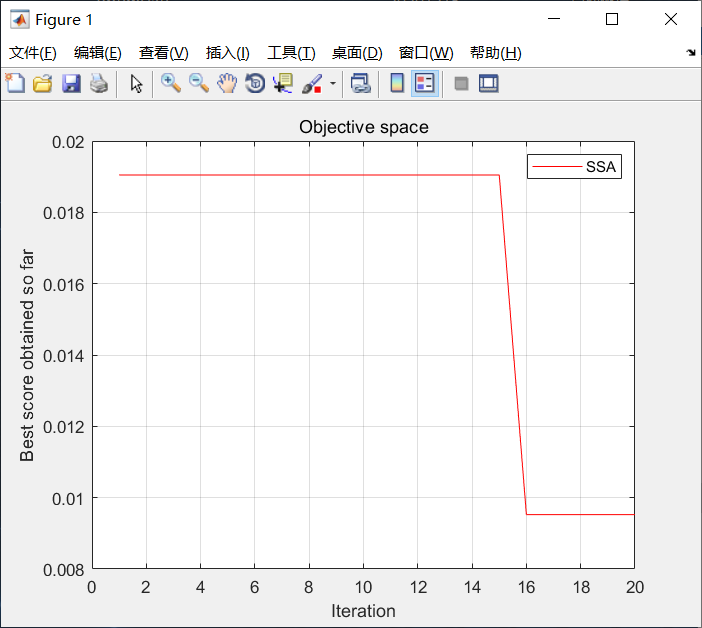
Figure 2 Convergence curve of Harris Eagle algorithm

Test statistics are shown in the following table

test result	Test Set Correctness Rate	Training Set Correctness Rate
BP Network	100%	95%
HHO-BP	100%	99.8%

6. References

Prediction of water resource demand in Ningxia based on BP network