Decision tree in sklearn
Module: sklearn.tree
| tree.DecisionTreeClassifier | Classification tree |
|---|---|
| tree.DecisionTreeRegressor | Regression tree |
| tree.export_graphviz | The generated decision tree is exported to DOT mode for drawing |
| tree.ExtraTreeClassifier | High random version classification tree |
| tree.ExtraTreeRegressor | High random version of regression tree |
Basic modeling process:
- Instantiate and establish evaluation model object
- Training model through model interface
- Extract the required information through the model interface
Take the classification tree as an example:
from skleran import tree #Import required modules
clf = tree.DecisionTreeClassifier() #instantiation
clf = clf.fit(X_train,y_train)#Training model with training set data
result = clf,score(x_test,y_test)#Import the test set and call the required information from the interface.
Of course, before modeling, we first need to obtain the data set, visualize the data, process the data, etc
1, DecisionTreeClassifier
1. Important parameters
1.1 criterion
In order to transform the table into a tree, the decision tree needs to find the best node and the best branching method. For the classification tree, the index to measure this "best" is called "impure". Theoretical knowledge of specific decision tree: Decision tree.
The Criterion parameter is used to determine the calculation method of impurity. skleran offers two options.
- Enter "entropy" to use information entropy.
- Enter "gini" to use gini coefficient.
Compared with Gini coefficient, information entropy is more sensitive to impure, and the punishment for impure is the strongest. However, in practice, the effects of information entropy and Gini coefficient are basically the same.
At the same time, because information entropy is more sensitive to impurity, when information entropy is used as an index, the growth of decision tree will be more "fine". Therefore, for high-dimensional data or data with a lot of noise, information entropy is easy to over fit, and the effect of Gini coefficient is often better in this case.
1.2 random_state & splitter
random_state is used to set the parameter of random mode in the branch. The default is None. Randomness will be more obvious in high dimensions.
splitter is also used to control the random options in the decision tree. Two input values are used to input "best". Although the decision tree is random in branching, it will give priority to more important features for branching. If you enter "random", the decision tree will be more random in branching, and the tree will be deeper and larger because it contains more unnecessary information, which may lead to over fitting problems. When you predict that your model may be over fitted, using these two parameters can help you reduce the possibility of over fitting after the tree is built. Of course, once the tree is built, we still use pruning parameters to prevent over fitting.
clf = tree.DecisionTreeClassifier(criterion='entropy',random_state = 30,splitter='random')
1.3 pruning parameters
Without any restriction, a decision tree will grow until the index measuring impurity is the best or there are no more features. Such decision trees often over fit.
In order to make the decision tree more generalized, sklearn provides different pruning strategies:
- max_depth
Limit the maximum depth of the tree and cut off all branches exceeding the set depth
The most extensive pruning parameter is very effective in high dimension and low sample size. In actual use, it is recommended to try from = 3 to see the fitting effect, and then decide whether to increase the set depth.
- min_samples_leaf & min_samples_split
min_samples_leaf defines that each child node of a node after branching must contain at least min_samples_leaf is a training sample, otherwise the branch will not occur, or the branch will contain min towards each child node_ samples_ Leaf occurs in the direction of two samples.
General collocation Max_ The use of depth will have a magical effect in the regression tree and make the model smoother. The number and size of this parameter will cause over fitting, which will prevent the model from learning data. In general, the build starts with = 5. If the sample size contained in the leaf node changes greatly, the input floating-point number is established as a percentage of the sample size. At the same time, this parameter can ensure the minimum size of each leaf, and can avoid low variance and over fitting leaf nodes in the regression problem. For classification problems with few categories, = 1 is usually the best choice.
min_samples_split limit: a node must contain at least min_samples_split training samples, this node is allowed to be branched, otherwise the branching will not occur.
- max_features & min_impurity_decreases
General fit max_depth is used as the "refinement" of the tree“
max_features limits the number of features considered when branching. Features exceeding the limit will be discarded, which is similar to max_depth.
If you want to prevent overfitting by dimensionality reduction, it is recommended to use PCA, ICA or dimensionality reduction algorithm in feature selection module.
min_impurity_decrease limits the size of information gain. Branches with information gain less than the set value will not occur.
- Confirm the optimal pruning parameters
Then how to determine what value to fill in for each parameter? At this time, we will use the curve to determine the super parameter to judge, and continue to use the trained decision tree model clf.
The learning curve of superparameter is a curve with the value of superparameter as the abscissa and the measurement index of the model as the ordinate. It is a line used to measure the performance of the model under different superparameter values. Our model measurement index is score.
import matplotlib.pyplot as plt
test = []
for i in range(10):
    clf = tree.DecisionTreeClassifier(max_depth=i+1
                                     ,criterion="entropy"
                                     ,random_state=30
                                     ,splitter="random"
                                     )
    clf = clf.fit(Xtrain, Ytrain)
    score = clf.score(Xtest, Ytest)
    test.append(score)
plt.plot(range(1,11),test,color="red",label="max_depth")
plt.legend()
plt.show()
2. Build a tree
1. Import the required algorithm libraries and modules
from sklearn import tree
from sklearn.datasets import load_wine
from sklearn.model_selection import train_test_split
2. Explore data
- Import data and view data types
wine = load_wine()
wine.data
array([[1.423e+01, 1.710e+00, 2.430e+00, ..., 1.040e+00, 3.920e+00,
        1.065e+03],
       [1.320e+01, 1.780e+00, 2.140e+00, ..., 1.050e+00, 3.400e+00,
        1.050e+03],
       [1.316e+01, 2.360e+00, 2.670e+00, ..., 1.030e+00, 3.170e+00,
        1.185e+03],
       ...,
       [1.327e+01, 4.280e+00, 2.260e+00, ..., 5.900e-01, 1.560e+00,
        8.350e+02],
       [1.317e+01, 2.590e+00, 2.370e+00, ..., 6.000e-01, 1.620e+00,
        8.400e+02],
       [1.413e+01, 4.100e+00, 2.740e+00, ..., 6.100e-01, 1.600e+00,
        5.600e+02]])
wine.target
# It can be seen that the three categories are 0, 1 and 2
array([0, 0, 0, 0, 0, 0, 0, 0, 0, 0, 0, 0, 0, 0, 0, 0, 0, 0, 0, 0, 0, 0,
       0, 0, 0, 0, 0, 0, 0, 0, 0, 0, 0, 0, 0, 0, 0, 0, 0, 0, 0, 0, 0, 0,
       0, 0, 0, 0, 0, 0, 0, 0, 0, 0, 0, 0, 0, 0, 0, 1, 1, 1, 1, 1, 1, 1,
       1, 1, 1, 1, 1, 1, 1, 1, 1, 1, 1, 1, 1, 1, 1, 1, 1, 1, 1, 1, 1, 1,
       1, 1, 1, 1, 1, 1, 1, 1, 1, 1, 1, 1, 1, 1, 1, 1, 1, 1, 1, 1, 1, 1,
       1, 1, 1, 1, 1, 1, 1, 1, 1, 1, 1, 1, 1, 1, 1, 1, 1, 1, 1, 1, 2, 2,
       2, 2, 2, 2, 2, 2, 2, 2, 2, 2, 2, 2, 2, 2, 2, 2, 2, 2, 2, 2, 2, 2,
       2, 2, 2, 2, 2, 2, 2, 2, 2, 2, 2, 2, 2, 2, 2, 2, 2, 2, 2, 2, 2, 2,
       2, 2])
For a more intuitive view of the dataset, import the pandas library
pd.concat([pd.DataFrame(wine.data),pd.DataFrame(wine.target)],axis=1)
	0	1	2	3	4	5	6	7	8	9	10	11	12	0
0	14.23	1.71	2.43	15.6	127.0	2.80	3.06	0.28	2.29	5.64	1.04	3.92	1065.0	0
1	13.20	1.78	2.14	11.2	100.0	2.65	2.76	0.26	1.28	4.38	1.05	3.40	1050.0	0
2	13.16	2.36	2.67	18.6	101.0	2.80	3.24	0.30	2.81	5.68	1.03	3.17	1185.0	0
3	14.37	1.95	2.50	16.8	113.0	3.85	3.49	0.24	2.18	7.80	0.86	3.45	1480.0	0
4	13.24	2.59	2.87	21.0	118.0	2.80	2.69	0.39	1.82	4.32	1.04	2.93	735.0	0
...	...	...	...	...	...	...	...	...	...	...	...	...	...	...
173	13.71	5.65	2.45	20.5	95.0	1.68	0.61	0.52	1.06	7.70	0.64	1.74	740.0	2
174	13.40	3.91	2.48	23.0	102.0	1.80	0.75	0.43	1.41	7.30	0.70	1.56	750.0	2
175	13.27	4.28	2.26	20.0	120.0	1.59	0.69	0.43	1.35	10.20	0.59	1.56	835.0	2
176	13.17	2.59	2.37	20.0	120.0	1.65	0.68	0.53	1.46	9.30	0.60	1.62	840.0	2
177	14.13	4.10	2.74	24.5	96.0	2.05	0.76	0.56	1.35	9.20	0.61	1.60	560.0	2
View the name of the feature
wine.feature_names
['alcohol',
 'malic_acid',
 'ash',
 'alcalinity_of_ash',
 'magnesium',
 'total_phenols',
 'flavanoids',
 'nonflavanoid_phenols',
 'proanthocyanins',
 'color_intensity',
 'hue',
 'od280/od315_of_diluted_wines',
 'proline']
View target classification
wine.target_names
array(['class_0', 'class_1', 'class_2'], dtype='<U7')
- Separate the data and select the training set and test set
The proportion of training set is 0.7 and the proportion of test set is 0.3
X_train,X_test,y_train,y_test = train_test_split(wine.data,wine.target,test_size=0.3)
3. Modeling
The information entropy is selected as the method to calculate the impurity
clf = tree.DecisionTreeClassifier(criterion = 'entropy')
Training model
clf = clf.fit(X_train,y_train)
View accuracy
score = clf.score(X_test,y_test)
# 0.9259259259259259
4. Painting tree
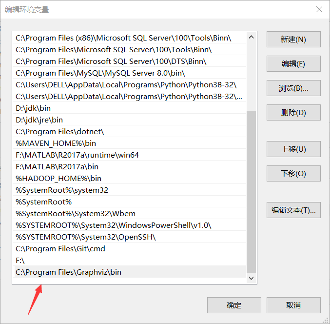
First, you need to install the graphviz library and go to Official website Download the app, otherwise the tree will not be displayed.
And add the path of the application in the environment variable.
"My computer > Properties > environment variables > Path > New > add path"
Installation library, using Tsinghua image
!pip install graphviz -i https://pypi.tuna.tsinghua.edu.cn/simple
After the above operations are completed, start to use this library to draw trees
tree.export_graphviz should provide a decision tree, the name of eigenvalue, the name of classification result, etc.
import graphviz
feature_name = ['alcohol','malic acid','ash','Alkalinity of ash','magnesium','Total phenol','flavonoid','Non flavane phenols','anthocyanin','Color intensity','tone','Diluted wine','proline']
dot_data = tree.export_graphviz(clf
                                ,feature_names=feature_name
                                ,class_names=['Gin','Shirley','Belmord']
                                ,filled=True
                                ,rounded=True)# fillet
graph = graphviz.Source(dot_data)
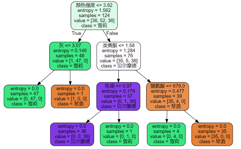
See the importance of different features
[*zip(feature_name,clf.feature_importances_)]
[('alcohol', 0.0),
 ('malic acid', 0.0),
 ('ash', 0.036209954705410934),
 ('Alkalinity of ash', 0.0),
 ('magnesium', 0.0),
 ('Total phenol', 0.0),
 ('flavonoid', 0.37359968306232505),
 ('Non flavane phenols', 0.0),
 ('anthocyanin', 0.0),
 ('Color intensity', 0.45986979793750715),
 ('tone', 0.034247526308054214),
 ('Diluted wine', 0.0),
 ('proline', 0.09607303798670264)]
5. Test the test set
score_test = clf.score(X_test,y_test)
score_test# Good performance
The above completes the generation of decision tree with sklearn. You can consider using more parameters to train the model and observe the impact of different parameters on the decision tree.
The above materials are mainly from the machine learning Sklearn class of vegetables.