Single Layer Perceptor

• Input Nodes: x1, x2, x3
• Output node:Y
• Weight vectors: w1, w2, w3
• Bias factor:b
• Activation function: f =sign(x), that is, f=1 when x > 0, f=1 when x < 0, f=0 when x = 0;

An example: [Comments, explanations in code]

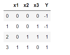
If B = 0.7, the input initial weights of x1, x2 and x3 are 0.5, 0.6 and 0.4, and the input data and labels are as follows:

testArray = np.array([[0,0,0,-1],
         [0,0,1,-1],
         [0,1,1,1],
         [1,1,0,1]])
import pandas as pd
testD = pd.DataFrame(testArray,index=None,columns=['x1','x2','x3','Y'])
testD

• Before the input is input to the neural network, it is processed by the initial weight, and then the output Y is processed by the activation function.
• The output Y is calculated as: when (x1 * 0.5 + x2 * 0.6 + X3 * 0.4-0.6) > 0, Y=1; when (x1 * 0.5 + x2 * 0.6 + X3 * 0.4-0.6) < 0, Y=1; when (x1* 0.5+x2* 0.6+x3* 0.4-0.6)=0, Y=0.

import tensorflow as tf
import numpy as np
import matplotlib.pyplot as plt
# Input data x1, x2, x3
X = np.array([[1,3,3],
            [1,4,3],
            [1,1,1]])

# Label
Y = np.array([1,1,-1])
# Weight initialization, 1 row, 3 columns, range - 1 ~ 1
W = (np.random.random(3)-0.5)*2
# print(W)
#Learning Rate Setting
learn_rate=0.11
# Number of iterations calculated
n=0
# Neural Network Output
output_y = 0
def update():
    global X,Y,W,learn_rate,n
    n+=1
    output_y = np.sign(np.dot(X,W.T))
    W_change = learn_rate*(Y-output_y.T).dot(X)/int(X.shape[0])
    W = W_change+W  #Changing parameter W equals weight
   
for _ in range(100):
    update()#Update weight
    print(W) #Print the current weight
    print(n) #Number of Print Iterations
    output_y = np.sign(np.dot(X,W.T)) #Calculate the current output
    if(output_y == Y.T).all(): #If the actual output equals the expected output, the model converges and the cycle ends.
        print("Finish!")
        print("epoch:[It has converged.",n)
        break

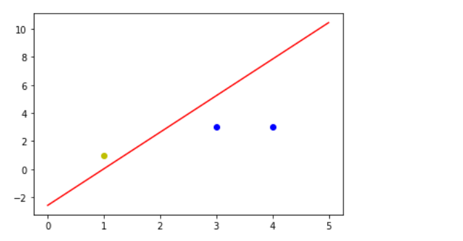
#Positive samples
x1 = [3,4]
y1 = [3,3]
#Negative sample
x2 = [1]
y2 = [1]

# Slope and Interception of Computer Boundary
k = -W[1]/W[2]
d = -W[0]/W[2]
print("k=",k)
print("d=",d)

xdata = np.linspace(0,5)
plt.figure()
plt.plot(xdata,xdata*k+d,'r')
plt.plot(x1,y1,'bo')
plt.plot(x2,y2,'yo')
plt.show()

Finally, the convergence tends to be stable after 12 iterations.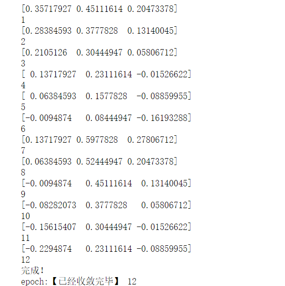

Observation graphics can effectively distinguish data: