1. Target determination
Using the volume of the market, the number of red stocks and the flow of funds from the north and the south, we can roughly observe the recent market heat. At the same time, from the technical level, we can also understand the current market trend combined with the K-line average. The operation of individual stocks can not be separated from the trend of the industry, nor can it be separated from the trend of the index plate. The resonance of the index results in the comprehensive trend of the market.
Through the analysis of the above data, we can get the response strategies of the market in the near future.
Second, data acquisition
Data acquisition, mainly through tushare acquisition. The data obtained include the data of the North-South funds, the basic data of the market and the data of the relevant index. After downloading, in order to extract data more conveniently and quickly, it can also be saved locally. Because the data acquired by tushare is mainly in DataFrame mode, it can easily carry out related operations, and many intermediate variables will be generated during the period, so it is not necessary to save all data, otherwise the workload is relatively large, and the significance is not too great. The final data obtained are summarized as follows: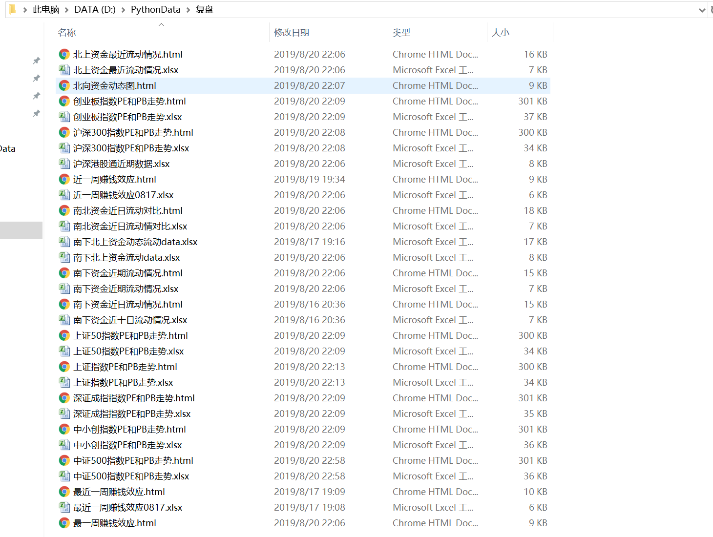
Third, data cleaning
In this processing, data cleaning mainly centers on data format. For missing data, we do not do alternative processing to maintain the continuity and authenticity of time series. For example, if we get the data of Hong Kong Stock Exchange, because of different holidays, the data may be missing, but it does not mean that it is bad data. It is inappropriate to delete it blindly. Some data cleaning and format conversion codes are as follows:
#Construction of Market Heat
#Recent Time Value
now=datetime.now()
st=now-6*Day()
Endtime=now
Endtime=Endtime.strftime("%Y%m%d")

dates=pd.date_range(st,periods=7)
date_str=dates.strftime('%Y%m%d')
date_str
EarningEffect_arr=[EarningEffect1,EarningEffect2,EarningEffect3,EarningEffect4,EarningEffect5,EarningEffect6,EarningEffect7]
EarningEffect_arr.reverse()
EarningEffect_arr=np.nan_to_num(EarningEffect_arr) #Here, the NAN value is set to 0, which is convenient for later drawing.
EarningEffect_arr=np.round(EarningEffect_arr,1)
EarningEffect_arr
4. Data collation and analysis
Part I: Analysis of the Money-making Effect
This part is mainly based on the recent turnover and the number of red plates (that is, today's closing price is higher than yesterday's closing price). By means of visualization, it reflects the trend. Because of the relatively large amount of code, the core part is extracted for analysis.
#Import related libraries for use in building systems.
import pandas as pd
import numpy as np
import matplotlib.pyplot as plt
from datetime import  datetime
from pandas.tseries.offsets import Day

import seaborn as sns
from pyecharts import Bar,Line,Grid,Overlap,Gauge
from pyecharts import online
online() # needed for online viewing
#The following solution is to use pyecharts for visualization
plt.rcParams['font.sans-serif']=['SimHei'] #Used for normal display of Chinese labels
plt.rcParams['axes.unicode_minus']=False #Used for normal negative sign display
#Save the 7-day market data.
df_dailys=[]
for i in range(0,7):
    df_dailys_temp=pro.daily(trade_date=date_str[i])
    df_dailys.append(df_dailys_temp)
At the same time, we need to save the market data, the implementation code of the penultimate seventh day of the CPC is given, and similar days are available. We define an array to save the daily earning effect.
#Money-making effect of the last seven days
D7_red_count=D7[D7.close>D7.pre_close].count().ts_code
D7_count=D7.ts_code.count()
EarningEffect7=(D7_red_count/D7_count*100)

#EarningEffect7=('%.2f' % (D7_red_count/D7_count*100))
#EarningEffect7=float(EarningEffect7)

EarningEffect_arr=[EarningEffect1,EarningEffect2,EarningEffect3,EarningEffect4,EarningEffect5,EarningEffect6,EarningEffect7]
EarningEffect_arr.reverse()
EarningEffect_arr=np.nan_to_num(EarningEffect_arr) #Here, the NAN value is set to 0, which is convenient for later drawing.
EarningEffect_arr=np.round(EarningEffect_arr,1)
EarningEffect_arr
Then, the earning effect data are saved first, and at the end of the first part, combined with the market heat, it is drawn in the same graph, combined with analysis, more direct and efficient.
Amount=[D7_amount,D6_amount,D5_amount,D4_amount,D3_amount,D2_amount,D1_amount]

Earn=list(EarningEffect_arr)
df_Amount_Earn=pd.DataFrame([date_str,Amount,Earn])
df_Amount_Earn=df_Amount_Earn.T
df_Amount_Earn=df_Amount_Earn.rename(columns={0:'date',1:'volume',2:'Money-making Temperature'})

df_Amount_Earn.to_excel('D:/PythonData/replay/Money-making effect in recent week 0817.xlsx')
The second half of the first part is the construction of market heat. We introduce pyecharts here and use overlap() to draw them together to achieve visualization. The results are as follows: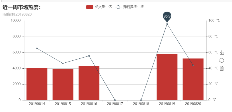
The first part ends here. In the first part, we quickly constructed a general picture of the recent revaluation. Then, we analyzed the important trend of the North-South funds.
Part II: North-South Funds Analysis
Here, we introduce the flow of funds from North and South to analyze the current attitude of the major players towards the current market, which can give us a further basis for decision-making. Its main implementation process is as follows:
attr=list(reversed(trade_date))

v1_temp=(Money_flow.hgt/100).round(1)
v1=list(reversed(v1_temp))

v2_temp=(Money_flow.sgt/100).round(1)
v2=list(reversed(v2_temp))

v3=(v1_temp+v2_temp).round(2)
v3=list(reversed(v3))

Money_flow_data=pd.DataFrame([attr,v1,v2,v3])
Money_flow_data.to_excel("D:/PythonData/Recent Capital Flow in North China.xlsx")

from pyecharts import Overlap

bar = Bar("Recent Capital Flow in North China","Hill Organization:"+str(Endtime))
line=Line("")
bar.add("Shanghai Stock Exchange", attr, v1, is_stack=True)
bar.add("Shenzhen Stock Exchange", attr, v2, is_stack=True)
line.add("Total inflow",attr, v3)

overlap=Overlap()
overlap.add(bar)
overlap.add(line)
The results are as follows: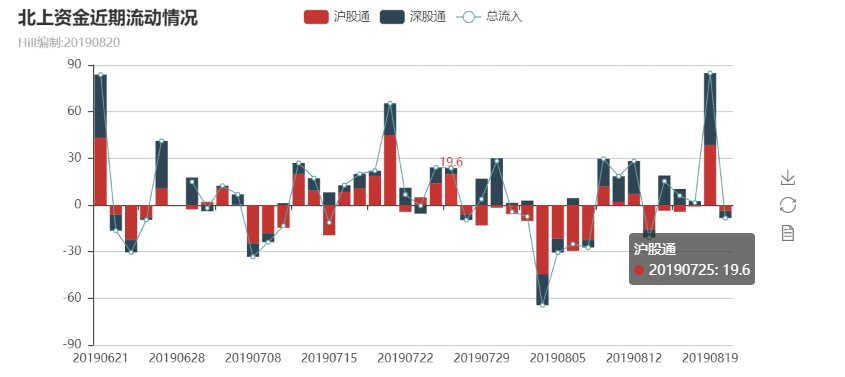
From the figure, we can see that the northward capital outflow on that day. This is also the coldness after overheating the previous day. For the observation of market sentiment, on the other hand, we can observe whether our own emotions are normal, and whether the decision-making is rational. At the same time, if we want to observe the flow of funds in different periods, we can set the window as a sliding mode. The main code is as follows:
days = Money_flow.trade_date
days_v1 = (Money_flow.north_money/100).round(1)
bar = Bar("Northward capital flow (sliding view)","Hill Organization:"+Endtime)
bar.add(
    "",
    days,
    days_v1,
    # Default X axis, horizontal
    is_datazoom_show=True,
    datazoom_type="slider",
    datazoom_range=[1, 30],
    # Additional data Zoom control bar, vertical
    is_datazoom_extra_show=True,
    datazoom_extra_type="slider",
    datazoom_extra_range=[-100, 100],
    is_toolbox_show=False,
    mark_line=['average'],
    mark_point=['max','min']
)
bar.render()
bar
Running, we can get the bar chart as follows: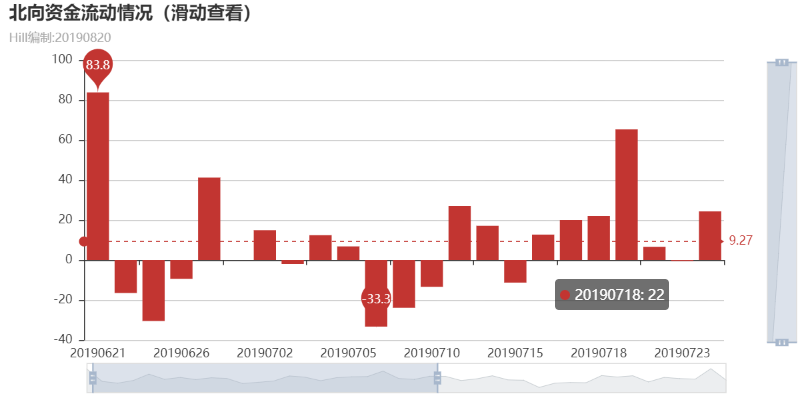
By sliding the data bar below, you can see the flow of funds in different dates. For example, if you only want to see about a week, you can slide the following time to 0714-0820. Through the data bar on the right side, you can see the time within the limit amount. If you only want to see more than 2 billion, you can slide below the toolbar to 2 billion. This analysis is more convenient, depending on the purpose of our analysis.
The following code can help us to see the specific ownership of northbound funds
#Having obtained the list of northbound shareholdings hk_hlod Shanghai, Shenzhen and Hong Kong Stock Exchange Detailed ratio Share Holdings, vol Holdings Number (Stocks)
SSH_stocks_all=pro.hk_hold(trade_date='20190819')

North_stocks_SH=pro.hk_hold(trade_date='20190819',exchange='SH')
North_stocks_SH.sort_values(by='ratio',inplace=True,ascending=False)

North_stocks_SZ=pro.hk_hold(trade_date='20190820',exchange='SZ')
North_stocks_SZ.sort_values(by='ratio',inplace=True,ascending=False)

North_stocks=pd.concat([North_stocks_SH,North_stocks_SZ])
North_stocks=North_stocks.sort_values(by='ratio',ascending=False)

North_stocks_SH
North_stocks_SZ
Some of the data are as follows: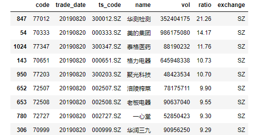
At the same time, if we want to view the top10 stock of that day, we can do it by the following code:
df_hsgt_SHtop10=pro.hsgt_top10(trade_date='20190820', market_type='1')
df_hsgt_SZtop10=pro.hsgt_top10(trade_date='20190820', market_type='3')
df_hsgt_SZtop10
df_hsgt_SHtop10.sort_values(by='net_amount',ascending=False)
In this way, we can get the top 10 shares of Shanghai Stock Exchange traded on the day of Beisheng: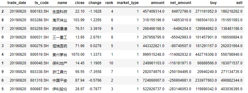
This concludes the second part.
Part III: Construction of Trend Scoring System
Trend score mainly gives the rating of each index. The rating is based on the strength of the average. The short-term average of 20 days and the long-term average of 200 days are selected as the reference, and the judgment is made according to the point position of the day. Its core code is as follows:
#The Shanghai Stock Exchange Index score: the lowest is 1 point, the highest is 6 points.

#6 is divided into multi-head interval; 5 is divided into multi-oscillation interval; 4 is divided into oscillation interval; 3 is divided into oscillation interval; 2 is divided into oscillation empty interval; 1 is divided into short interval.
SHZ_Year=pro.index_daily(ts_code='000001.SH',start_date=Yeartime,end_date=Endtime).close.mean()
SHZ_Twenty=pro.index_daily(ts_code='000001.SH',start_date=TwentyDaystime,end_date=Endtime).close.mean()

SHZ_today=pro.index_daily(ts_code='000001.SH')
SHZ_today=SHZ_today.iloc[0,2]

#If you can't find the right switch, use if_else instead.
if (SHZ_today>SHZ_Twenty)&(SHZ_Twenty>SHZ_Year):  #This means that the Shanghai Stock Exchange Index is currently above the 20-day average, while the 20-day average is above the annual line, with a multi-headed space with a score of max=6.
    rank_SHZ=6
elif (SHZ_today>SHZ_Year)&(SHZ_Year>SHZ_Twenty):
    rank_SHZ=5
elif (SHZ_Twenty>SHZ_today)&(SHZ_today>SHZ_Year):
    rank_SHZ=4
elif (SHZ_Year>SHZ_today)&(SHZ_today>SHZ_Twenty):
    rank_SHZ=3
elif (SHZ_Twenty>SHZ_Year)&(SHZ_Year>SHZ_today):
    rank_SHZ=2
else:
    rank_SHZ=1

print(rank_SHZ)
The above code gives the rating of the Shanghai Stock Exchange Index. Similar methods can be used to achieve the other six indexes. If Shenzhen synthesizes the index, as follows:
#Shenzhen stock index score:
SZC_Year=pro.index_daily(ts_code='399001.SZ',start_date=Yeartime,end_date=Endtime).close.mean()
SZC_Twenty=pro.index_daily(ts_code='399001.SZ',start_date=TwentyDaystime,end_date=Endtime).close.mean()

SZC_today=pro.index_daily(ts_code='399001.SZ')
SZC_today=SZC_today.iloc[0,2]

if (SZC_today>SZC_Twenty)&(SZC_Twenty>SZC_Year):  #This means that the Shanghai Stock Exchange Index is currently above the 20-day average, while the 20-day average is above the annual line, with a multi-headed space with a score of max=6.
    rank_SZC=6
elif (SZC_today>SZC_Year)&(SZC_Year>SZC_Twenty):
    rank_SZC=5
elif (SZC_Twenty>SZC_today)&(SZC_today>SZC_Year):
    rank_SZC=4
elif (SZC_Year>SZC_today)&(SZC_today>SZC_Twenty):
    rank_SZC=3
elif (SZC_Twenty>SZC_Year)&(SZC_Year>SZC_today):
    rank_SZC=2
else:
    rank_SZC=1

print(rank_SZC)
Repeat the steps above, and we can get the scores of seven important indices.
Finally, we give a comprehensive score:
Firstly, market value is used as weight:
ranks=np.array([rank_SHZ,rank_SZC,rank_CYB,rank_ZXC,rank_SZ50,rank_HS300,rank_ZHZ500])
#Empowerment in the form of market value can be done in other ways.
#8-17 Corresponding Total Market Value ($100 million): CS 500:74209; Shanghai: 319899; Shanghai and Shenzhen 300:350223; Shanghai 50:198903; Shenzhen: 204195; Entrepreneurship: 51775; Small and Medium-sized Ventures: 85129
ranks_Amount=np.array([319899,204195,51775,85129,198903,350223,319899])
ranks_Amount_sum=ranks_Amount.sum()
ranks_Amount_power=ranks_Amount/ranks_Amount_sum

print(ranks_Amount)
print(ranks_Amount_power)
print(ranks)
#The score is obtained by multiplying rating by weight.
rank=ranks_Amount_power*ranks
TrendRank=rank.sum()
TrendRank=round(TrendRank,2)
print(TrendRank)
The results are as follows: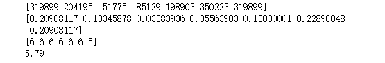
In another way, we can get inconsistent results by using the volume of the day. There is no absolute standard. We just hope to find a reference for empowerment. Utilizing the turnover, as follows:
#Take the volume of the day as the weight assignment
#Shanghai Stock Index 000001.SH Shanghai-Shenzhen 300 Index 000300.SH, Shanghai 50 000016.SH
#Shenzhen Composite Index 399001.SZ Small and Medium-sized Ventures 399005.SZ GEM 399006.SZ China Composite 500 Index 399905
df_float_mv = pro.index_dailybasic(trade_date='20190816', fields='ts_code,trade_date,float_mv,pe')
print(df_float_mv)

now_float_mv1=df_float_mv[df_float_mv.ts_code=='000001.SH'].float_mv
now_float_mv2=df_float_mv[df_float_mv.ts_code=='399001.SZ'].float_mv
now_float_mv3=df_float_mv[df_float_mv.ts_code=='399006.SZ'].float_mv
now_float_mv4=df_float_mv[df_float_mv.ts_code=='399005.SZ'].float_mv
now_float_mv5=df_float_mv[df_float_mv.ts_code=='000016.SH'].float_mv
now_float_mv6=df_float_mv[df_float_mv.ts_code=='000300.SH'].float_mv
now_float_mv7=df_float_mv[df_float_mv.ts_code=='399905.SZ'].float_mv  #This extraction method has middle brackets

now_float_need=np.array([now_float_mv1.values,now_float_mv2.values,now_float_mv3.values,
                         now_float_mv4.values,now_float_mv5.values,now_float_mv6.values,now_float_mv7.values])

now_float_need=np.array(now_float_need).flatten()  #Remove brackets from ndarray

now_float_need_sum=np.sum(now_float_need)
now_float_power=now_float_need/now_float_need_sum

print(ranks)
print(now_float_power)# after flatten

TrendRank_Float=np.sum(ranks*now_float_power)
TrankRenk_Float=np.round(TrendRank_Float,2)
TrankRenk_Float
The results are as follows: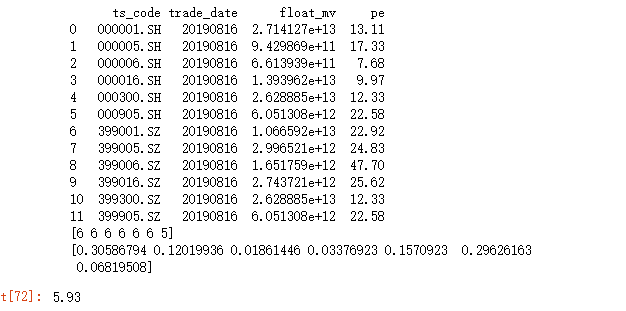
Visualization of grading:
Visualization of final reference positions: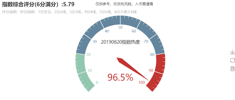
So far, our data collation and analysis has come to an end.
Part V: Insights and conclusions
The source of data can be either from the base book or from the technical side.
Fundamental data, from top to bottom, can be at the macroeconomic level, can also be at the industry level, and can be at the micro-enterprise level. Different dimensions of data analysis can be used, depending on our criteria for judging the market.
Technical data, from far to near, from near to far, can be extracted, long, medium and short period of data, also depends on our analysis objectives.
After extracting the data, we need to choose the dimension we value to think about, whether we care about the proportion, or the trend, or the relationship between each other, which needs to be considered in combination with the business level.
Concerned about trends, we can take the time series as the horizontal axis and the vertical axis to list the changing trends of the time we care about.
Concerned about proportion, we can show the relationship between the whole and the individual through pie chart and so on.
Concern relationship can be calculated by covariance, correlation coefficient and other items, and correlation can be analyzed by positive and negative size.
Through the trend map, we can see our conclusions. There is not much discussion here. Relevant explanations are given in the chart.
Insufficient:
Considering a point here, we can predict the change of the trend through the correlation resonance history of the trend line.
This belongs to the content of regression and prediction, but it is not here for the time being.
If you need specific code, or analysis process, or if you don't understand the chart clearly, you can contact me.
Emai:cug_ljx@163.com