Simple understanding of Gaussian distribution

The explanation in Baidu Encyclopedia is called "normal distribution", also known as normal distribution. If the random variable x obeys a normal distribution of mathematical expectation μ and variance σ 2, it is recorded as N (μ, σ 2). Its probability density function is the expected value μ of the normal distribution, which determines its position, and its standard deviation σ determines the range of distribution. When μ = 0, σ = 1, the normal distribution is the standard normal distribution.

One dimensional normal distribution

If the random variable X obeys a position parameter μ, the scale parameter is the probability distribution of σ, and its probability density function is: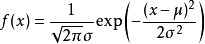

Then this random variable is called normal random variable. The distribution that normal random variable obeys is normal distribution. It is recorded as X-N (μ, σ 2), read as X obeys N (μ, σ 2), or X obeys normal distribution.
There are two parameters in the normal fraction, the spot expectation μ and the standard deviation σ, σ 2 is the variance
Normal distribution is the distribution of continuous random variables with two parameters μ and σ 2. The first parameter μ is the mean value of random variables subject to normal distribution, and the second parameter σ 2 is the variance of this random variable, so the normal distribution is recorded as N (μ, σ 2)
μ is the position parameter of normal distribution, which describes the centralized trend position of normal distribution. The probability rule is that the probability of taking the value close to μ is higher, while the probability of taking the value farther away from μ is lower. The normal distribution takes X = μ as the axis of symmetry and is completely symmetric left and right. The expectation, mean, median and mode of normal distribution are the same, all equal to μ.
σ describes the dispersion degree of data distribution of normal distribution. The larger σ is, the more scattered the data distribution is. The smaller σ is, the more concentrated the data distribution is. Also known as the shape parameter of normal distribution, the larger σ is, the flatter the curve is. On the contrary, the smaller σ is, the thinner the curve is.

Standard normal distribution

When μ = 0, σ = 1, the normal distribution is called the standard normal distribution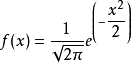

Its image looks like this!!!!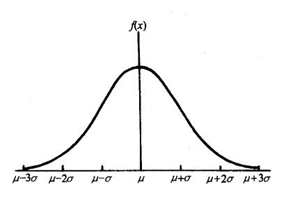
The normal distribution of elements has the following rules:
The larger σ is, the flatter the graph is, and the greater the data dispersion degree is; the smaller σ is, the thinner the graph is, and the smaller the data dispersion degree is.
About 69.27% of the samples fall between (μ - σ, μ + σ) (μ - σ, μ + σ)
About 95% of samples fall between (μ − 2 σ, μ + 2 σ) (μ − 2 σ, μ + 2 σ)
About 99% of samples fall between (μ - 3 σ, μ + 3 σ) (μ - 3 σ, μ + 3 σ)

Characteristics of normal distribution:
Concentration: the highest peak of the curve is in the center, and the position is where the mean is.
Symmetry: the normal distribution curve is symmetrical left and right with the position of the mean as the center, and the two ends of the curve are infinitely close to the transverse axis.
Uniform variability: the normal distribution curve drops evenly to the left and right sides with the position of the mean as the center.
The total area between the curve and the horizontal axis is equal to 1.
Example:



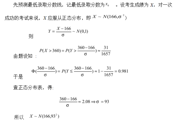
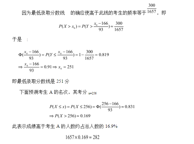
That is to say, candidate A is about 283, 251 points higher than the admission score limit, so candidate A can be admitted, but his ranking is 283, after 280, so he can't be admitted as A formal worker, only A temporary worker
Thesis link
See how python implements Gaussian distribution:
Direct code

import numpy as np
import matplotlib.pyplot as plt

#mean value
def average(data):
    return np.sum(data)/len(data)
#standard deviation
def sigma(data,avg):
    sigma_squ=np.sum(np.power((data-avg),2))/len(data)
    return np.power(sigma_squ,0.5)
#Probability of Gaussian distribution
def prob(data,avg,sig):
    print(data)
    sqrt_2pi=np.power(2*np.pi,0.5)
    coef=1/(sqrt_2pi*sig)
    powercoef=-1/(2*np.power(sig,2))
    mypow=powercoef*(np.power((data-avg),2))
    return coef*(np.exp(mypow))
#sample data
data=np.array([0.79,0.78,0.8,0.79,0.77,0.81,0.74,0.85,0.8
               ,0.77,0.81,0.85,0.85,0.83,0.83,0.8,0.83,0.71,0.76,0.8])
#The average number of Gaussian distribution based on sample data
ave=average(data)
#Standard deviation of Gaussian distribution from samples
sig=sigma(data,ave)
#Get data
x=np.arange(0.5,1.0,0.01)

p=prob(x,ave,sig)
plt.plot(x,p)
plt.grid()
plt.xlabel("apple quality factor")
plt.ylabel("prob density")
plt.yticks(np.arange(0,12,1))
plt.title("Gaussian distrbution")
plt.show()

Let's see what the generated image looks like: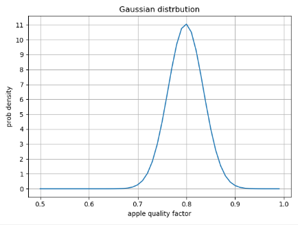

It can be seen that when the average value is 0.8, approximately equal to 0.8, the probability density at 0.8-0.7 is very small
So the data set is between 0.7-0.9, and the maximum value is 0.8.
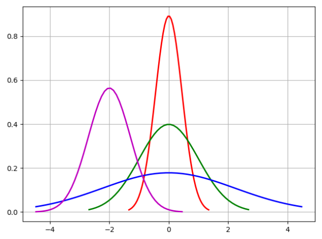
Drawing probability density function of normal distribution

import math
import numpy as np
import matplotlib.pyplot as plt
#
# Python implementation of normal distribution
# Drawing probability density function of normal distribution
u = 0  # Mean Mu
u01 = -2
sig = math.sqrt(0.2)  # Standard deviation Delta
sig01 = math.sqrt(1)
sig02 = math.sqrt(5)
sig_u01 = math.sqrt(0.5)
x = np.linspace(u - 3 * sig, u + 3 * sig, 50)
x_01 = np.linspace(u - 6 * sig, u + 6 * sig, 50)
x_02 = np.linspace(u - 10 * sig, u + 10 * sig, 50)
x_u01 = np.linspace(u - 10 * sig, u + 1 * sig, 50)
y_sig = np.exp(-(x - u) ** 2 / (2 * sig ** 2)) / (math.sqrt(2 * math.pi) * sig)
y_sig01 = np.exp(-(x_01 - u) ** 2 / (2 * sig01 ** 2)) / (math.sqrt(2 * math.pi) * sig01)
y_sig02 = np.exp(-(x_02 - u) ** 2 / (2 * sig02 ** 2)) / (math.sqrt(2 * math.pi) * sig02)
y_sig_u01 = np.exp(-(x_u01 - u01) ** 2 / (2 * sig_u01 ** 2)) / (math.sqrt(2 * math.pi) * sig_u01)
plt.plot(x, y_sig, "r-", linewidth=2)
plt.plot(x_01, y_sig01, "g-", linewidth=2)
plt.plot(x_02, y_sig02, "b-", linewidth=2)
plt.plot(x_u01, y_sig_u01, "m-", linewidth=2)
# plt.plot(x, y, 'r-', x, y, 'go', linewidth=2,markersize=8)
plt.grid(True)
plt.show()

We have looked up a lot of data to explain the Gaussian distribution too much. We only write a little here. For details, please refer to Normal Distrbution