Histogram based on OpenCV4

Image histogram is an important statistical feature of an image. It represents the statistical relationship between each gray level in a digital image and the frequency of the gray level (the number of gray levels). According to the definition of histogram, it can be expressed as:
P ( r k ) = n k N ( k = 0 , 1 , 2 , ⋯   , L − 1 ) P(r_k)=\frac{n_k}{N} \qquad (k=0,1,2,\cdots ,L-1) P(rk​)=Nnk​​(k=0,1,2,⋯,L−1)
Where: N N N is the total number of pixels of an image; n k n_k nk ， is the second k k Number of pixels of k-level gray scale; r k r_k rk ， is the second k k k gray level; L L L is the gray level series; P ( r k ) P(r_k) P(rk) is the probability of occurrence of the gray level.
Histogram has the following properties:
(1) Histogram is a one-dimensional information description of an image
In the histogram, it can only reflect the gray range, gray level distribution and average brightness of the whole image, but can not reflect the position of a gray value pixel of the image, so it loses the two-dimensional feature of the image.
(2) The mapping relationship between gray histogram and image is not unique
This property can be based on property 1. Since the histogram does not contain spatial location information, one gray histogram can correspond to multiple images, but one image can only correspond to one gray histogram.

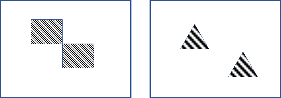
For example, the above two images correspond to the same gray histogram when the number of gray pixels is the same.
(3) The histogram satisfies the superposition
If we know the histogram of each region after the histogram is divided into several regions, we can add them together to get the histogram of the image.

We often calculate and draw histogram based on opencv.
OpenCV4 provides the function cv.calcHist(), which can count the number of each pixel in the image:

hist=cv.calcHist(images,channels,mask,histSize,ranges,hist,accumulate)

• Images: image array of histogram to be counted. All images in the array should have the same size and data type, and the data type can only be CV_8U,CV_16U and CV_32F is one of the three, but the number of channels of different images can be different.
• channels: the channel index array to be counted. The channel index of the first image is from 0 to images[0].channels()-1, the second image channel index is from images[0].channels() to images[0].channels()+ images[1].channels()-1, and so on.
• Mask: optional operation mask. If the matrix is empty, it means that pixels at all positions in the image are included in the histogram. If the matrix is not empty, it must be the same size as the input image and the data type is CV_8U.
• hist: the output statistical histogram result is an array of dims dimensions.
• ranges: the range of gray values in each image channel
• Accumulate: the flag of whether to accumulate statistical histograms. If accumulate (true), the statistical results of previous images will not be cleared when counting the histograms of new images. The same function is mainly used to count the histograms of multiple images as a whole.
  After calling this function, we can get the pixel frequency of any gray level in the image. We can draw the gray histogram of the generated sequence based on the Matplotlib library.

import cv2 as cv
import sys
import numpy as np
from matplotlib import pyplot as plt
np.set_printoptions(suppress=True)

if __name__=='__main__':
    #For the three channel images read here, we need to process each channel separately when calculating the gray histogram
    image=cv.imread('OIP-C.jfif')
    cv.imshow('image',image)

    if image is None:
        print("Failed to read image")
        sys.exit()
    color=('r','g','b')
    for i,col in enumerate(color):
        #Here hist is the pixel frequency of each channel. If the probability value is required, it needs to be divided by the total number of pixels of each channel
        hist = cv.calcHist([image], [i], None, [256], [0, 256])*3/image.size
        plt.plot(hist,color=col)
    #_,_,_=plt.hist(x=image.ravel(),bins=256,range=[0,256])
    cv.imshow('image',image)
    plt.show()
    cv.waitKey(0)
    cv.destroyAllWindows()

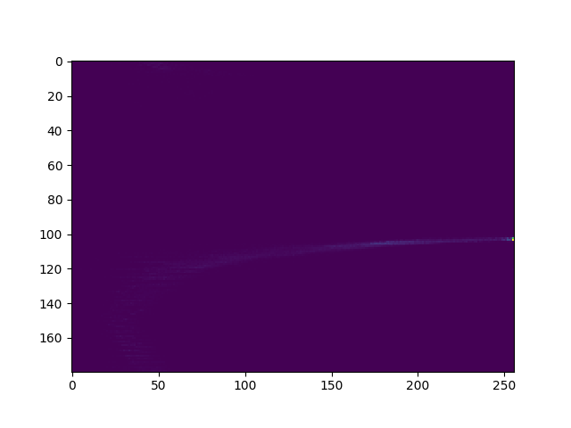
For color images, only considering the gray histogram can not meet our needs, so we usually consider the hue and saturation of the image, and make 2D histogram statistics according to the two features.
Similar to the calculation of one-dimensional histogram, the calculation of 2D histogram also uses the function cv.calcHist() function, but before calculation, the image needs to be converted from BGR format to HSV format, and several parameters need to be modified accordingly. Among them, channels means that h and S channels need to be counted, and the value is [0,1];histSize is [180256], where 180 represents H channel and 256 represents S channel; ranges is [0180,0256]

import cv2 as cv
import sys
import numpy as np
from matplotlib import pyplot as plt
np.set_printoptions(suppress=True)

if __name__=='__main__':
    #For the three channel images read here, we need to process each channel separately when calculating the gray histogram
    image=cv.imread('OIP-C.jfif')
    cv.imshow('image',image)
    image_hsv=cv.cvtColor(image,cv.COLOR_BGR2HSV)

    if image is None:
        print("Failed to read image")
        sys.exit()


    #Here hist is the pixel frequency of each channel. If the probability value is required, it needs to be divided by the total number of pixels of each channel
    hist = cv.calcHist([image_hsv], [0,1], None, [180,256], [0,180,0,256])
    plt.imshow(image_hsv)
    #_,_,_=plt.hist(x=image.ravel(),bins=256,range=[0,256])
    plt.imshow(hist,interpolation='nearest')
    plt.show()
    cv.waitKey(0)
    cv.destroyAllWindows()

The 2D histogram is generated as follows: