1. LeNet model

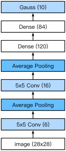
LeNet is divided into convolution layer block and full connection layer block. We will introduce the two modules respectively.

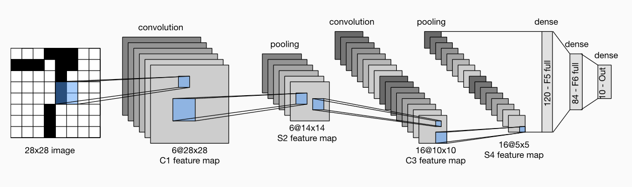
The basic unit in the convolution layer block is the convolution layer followed by the average pooling layer: the convolution layer is used to identify spatial patterns in the image, such as lines and local objects, and the average pooling layer after the convolution layer is used to reduce the sensitivity of the convolution layer to location.

The convolution layer block consists of two such basic units stacked repeatedly. In the convolution layer block, each convolution layer uses a 5 × 55 \times 55 × 5 window, and the sigmoid activation function is used on the output. The number of output channels of the first convolution layer is 6, and the number of output channels of the second convolution layer is increased to 16.

The full connection layer block includes three full connection layers. Their output numbers are 120, 84 and 10 respectively, where 10 is the number of output categories.

2. PyTorch implementation

2.1 model implementation

We implement the LeNet model through the Sequential class.

# Import the corresponding package
import sys
sys.path.append("/home/kesci/input")
import d2lzh1981 as d2l
import torch
import torch.nn as nn
import torch.optim as optim
import time

# Flatten operation, change dimension
class Flatten(torch.nn.Module):  
    def forward(self, x):
        return x.view(x.shape[0], -1)
# Reshape image size
class Reshape(torch.nn.Module): 
    def forward(self, x):
        return x.view(-1,1,28,28)      #(B x C x H x W)
 # Implementation of LeNet
net = torch.nn.Sequential( 
	# Resize image                                                 
    Reshape(),
    # The first convolution layer, input channel number 1, output channel number 6, convolution kernel size 5 * 5, filling 2
    nn.Conv2d(in_channels=1, out_channels=6, kernel_size=5, padding=2), #b*1*28*28  =>b*6*28*28
    # Activation function via sigmoid
    nn.Sigmoid(),   
    # Average pool layer, core size 2 * 2, step 2                                                    
    nn.AvgPool2d(kernel_size=2, stride=2),                              #b*6*28*28  =>b*6*14*14
    # In the second convolution layer, input channel is 6, output channel is 16, convolution core is 5 * 5
    nn.Conv2d(in_channels=6, out_channels=16, kernel_size=5),           #b*6*14*14  =>b*16*10*10
     # Activation function via sigmoid
    nn.Sigmoid(),
     # Average pool layer, core size 2 * 2, step 2  
    nn.AvgPool2d(kernel_size=2, stride=2),                              #b*16*10*10  => b*16*5*5
    # Flattening operation
    Flatten(),                                                          #b*16*5*5   => b*400
    # The first layer is fully connected to the hidden layer. The input dimension is 16 * 5 * 5, and the output dimension is 120
    nn.Linear(in_features=16*5*5, out_features=120),
    # Activation function via sigmoid
    nn.Sigmoid(),
    # The second layer is full connection hidden layer, with input dimension of 120 and output dimension of 84
    nn.Linear(120, 84),
     # Activation function via sigmoid
    nn.Sigmoid(),
    # The third layer is fully connected to the output layer, with the input dimension of 84 and the output dimension of 10
    nn.Linear(84, 10)
)

In LeNet, the height and width of the input in the convolution layer block decrease layer by layer. The convolution layer reduces the height and width by 4, while the pooling layer reduces the height and width by half, but the number of channels increases from 1 to 16. Full connection layer reduces the number of outputs layer by layer until the number of categories of the image becomes 10.

2.2 data acquisition and training

Let's implement the LeNet model. We still use fashion MNIST as the training data set.

# 256 data batches
batch_size = 256
# Get training data and test data
train_iter, test_iter = d2l.load_data_fashion_mnist(
    batch_size=batch_size, root='/home/kesci/input/FashionMNIST2065')

Select GPU for training, if there is no GPU, still use CPU for training

def try_gpu():
    """If GPU is available, return torch.device as cuda:0; else return torch.device as cpu."""
    if torch.cuda.is_available():
        device = torch.device('cuda:0')
    else:
        device = torch.device('cpu')
    return device

device = try_gpu()

We implement the evaluate ﹣ accuracy function, which is used to calculate the accuracy of the model net on the dataset data ﹣ ITER.

#Calculation accuracy
'''
(1). net.train()
  //Enable BatchNormalization and Dropout and set BatchNormalization and Dropout to True
(2). net.eval()
//Do not enable BatchNormalization and Dropout, set BatchNormalization and Dropout to False
'''

def evaluate_accuracy(data_iter, net,device=torch.device('cpu')):
    """Evaluate accuracy of a model on the given data set."""
    acc_sum,n = torch.tensor([0],dtype=torch.float32,device=device),0
    for X,y in data_iter:
        # If device is the GPU, copy the data to the GPU.
        X,y = X.to(device),y.to(device)
        net.eval()
        with torch.no_grad():
            y = y.long()
            acc_sum += torch.sum((torch.argmax(net(X), dim=1) == y))  #[[0.2 ,0.4 ,0.5 ,0.6 ,0.8] ,[ 0.1,0.2 ,0.4 ,0.3 ,0.1]] => [ 4 , 2 ]
            n += y.shape[0]
    return acc_sum.item()/n

We define the function train to train the model.

'''
//Parameter meaning:
net: Network to train
train_iter: Training set
test_iter: Test set
criterion: loss function
num_epochs: Training cycle
batch_size: Number of small batch samples for training
device: Training device CPU perhaps GPU
lr: Learning rate
'''
def train_ch5(net, train_iter, test_iter,criterion, num_epochs, batch_size, device,lr=None):
    """Train and evaluate a model with CPU or GPU."""
    print('training on', device)
    net.to(device)
    # Random gradient reduced to optimization function
    optimizer = optim.SGD(net.parameters(), lr=lr)
    for epoch in range(num_epochs):
    	# Initialize various variables
        train_l_sum = torch.tensor([0.0],dtype=torch.float32,device=device)
        train_acc_sum = torch.tensor([0.0],dtype=torch.float32,device=device)
        n, start = 0, time.time()

		# Start training
        for X, y in train_iter:
            net.train()
            # Zero gradient parameter
            optimizer.zero_grad()
            X,y = X.to(device),y.to(device) 
            # Y? Hat is the output value of the network
            y_hat = net(X)
            # Calculated loss
            loss = criterion(y_hat, y)
            # Back propagation
            loss.backward()
            # Update parameters
            optimizer.step()
            
            with torch.no_grad():
            	# Convert to long
                y = y.long()
                # Sum of calculated losses
                train_l_sum += loss.float()
                # Calculate the correct number of predictions
                train_acc_sum += (torch.sum((torch.argmax(y_hat, dim=1) == y))).float()
                n += y.shape[0]
        test_acc = evaluate_accuracy(test_iter, net,device)
        print('epoch %d, loss %.4f, train acc %.3f, test acc %.3f, '
              'time %.1f sec'
              % (epoch + 1, train_l_sum/n, train_acc_sum/n, test_acc,
                 time.time() - start))

We reinitialize the model parameters to the corresponding device(cpu or cuda:0), and use Xavier for random initialization. Loss function and training algorithm still use cross entropy loss function and small batch random gradient descent.

# train
lr, num_epochs = 0.9, 10

def init_weights(m):
    if type(m) == nn.Linear or type(m) == nn.Conv2d:
        torch.nn.init.xavier_uniform_(m.weight)

net.apply(init_weights)
net = net.to(device)
#Cross entropy describes the distance between two probability distributions. The more cross entropy is, the closer they are
criterion = nn.CrossEntropyLoss()   
train_ch5(net, train_iter, test_iter, criterion,num_epochs, batch_size,device, lr)

The output result is: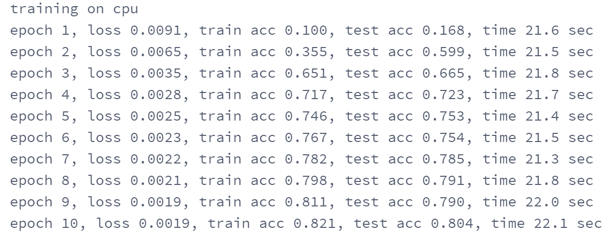

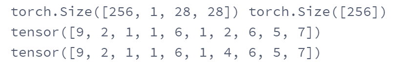
Test the trained network:

# test
for testdata,testlabe in test_iter:
    testdata,testlabe = testdata.to(device),testlabe.to(device)
    break
print(testdata.shape,testlabe.shape)
net.eval()
y_pre = net(testdata)
print(torch.argmax(y_pre,dim=1)[:10])
print(testlabe[:10])

The test results are as follows: