First of all, understand what is return. The purpose of regression is to predict the target value of another numerical data through several known data.

Suppose that the characteristic and the result satisfy the linear relation, that is to say, the independent variable of the formula is the known data x, and the function value h(x) is the target value to be predicted. This formula is called regression equation, and the process of getting this equation is called regression.

Suppose that the house area and the number of bedrooms are independent variables X, x1 is the house area, x2 is the number of bedrooms; the transaction price of the house is the dependent variable y, we use h(x) to express y. Suppose that the housing area, the number of bedrooms and the transaction price are linear.

They satisfy the formula

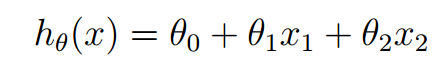
Theta in the above formula is a parameter, also known as weight, which can be understood as the influence degree of x1 and x2 on h(x). A little change to this formula is

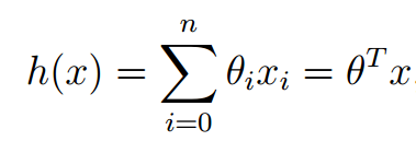
In the formula, both θ and x can be regarded as vectors, and n is the number of features.

If we predict h(x) according to this formula, X in the formula is known (characteristic value in the sample), but the value of θ is unknown. As long as we solve the value of θ, we can make prediction according to this formula.

Least Mean squares

Before we introduce LMS, we need to understand the concept of loss function.

What we should do is to select the optimal θ according to our training set, and make h(x) as close to the real value as possible in our training set. We define a function to describe the gap between h(x) and the real value. This function is called loss function. The expression is as follows:

The loss function here is the famous least square loss function. There is also a concept called the least square method, which will not be expanded here. We want to choose the optimal theta so that h(x) is nearest to the real value. This problem is transformed into solving the optimal θ, so that the loss function J(θ) takes the minimum value. (there are many other types of loss functions)

So how to solve the problem after transformation? This involves another concept: LMS and gradient descent.

LMS is the theoretical basis for obtaining the h(x) regression function, and the best parameter is obtained by minimizing the mean square error.

gradient descent

We ask for the solution to make J(θ) the minimum value of θ. The general idea of gradient descent algorithm is: first, we randomly give θ an initial value, then change the value of θ to make the value of J(θ) smaller, and repeat the process of changing θ to make J(θ) smaller until J(θ) is about equal to the minimum value.

First, we give an initial value of θ, and then update the value of θ in the direction where J(θ) changes the most, so we iterate. The formula is as follows:

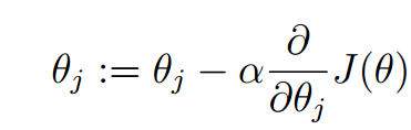
In the formula, α is called learning rate, which controls the change range of θ in each iteration to the direction of J(θ) becoming smaller. The derivative of J(θ) to θ indicates the direction of the greatest change of J(θ). Since the minimum value is obtained, the gradient direction is the reverse direction of the partial derivative.

• If the value of α is too small and the convergence speed is too slow, it may Overshoot the minimum.
• The closer to the minimum, the slower the descent speed
• Convergence: when the difference between the last two iterations is less than a certain value, the iteration ends

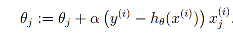
Solve the partial derivative as follows:

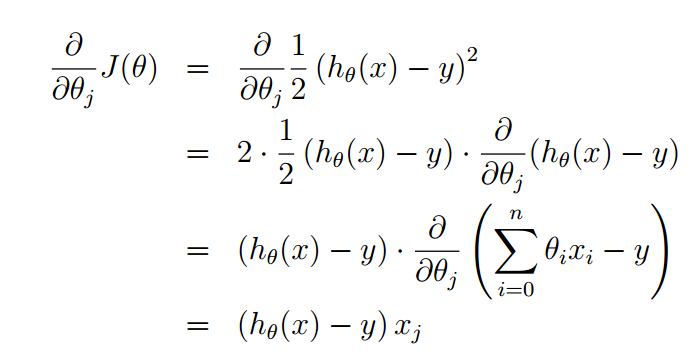
Then the iterative formula of theta becomes:

The above expression is only applicable when there is only one sample, so how to calculate the prediction function when there are m sample values? Batch gradient descent algorithm and random gradient descent algorithm

Batch gradient descent algorithm (BGD)

In the previous section, the parameter calculation formula of a single sample is transformed into the following expression for processing multiple samples:

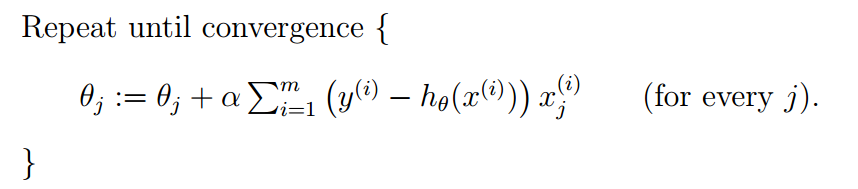
This new expression requires all training set data for each step of calculation, so it is called batch gradient descent.

Note that gradient descent may lead to local optimization, but in the optimization problem, we have proved that linear regression has only one best, because the loss function J(θ) is a quadratic convex function, which will not lead to local optimization. (assuming that the learning step α is not particularly large)

The execution process of the algorithm of batch gradient descent is as follows:

Look at the mathematical expression of batch gradient descent carefully. Each iteration requires the sum of all data set samples. The calculation amount will be very large, especially when the training data set is particularly large. Is there a method with less calculation and good effect? yes! This is: stochastic gradient descent (SGD)

Random gradient descent algorithm (SGD)

When calculating the direction of the fastest descent, the random gradient descent selects one data at random for calculation instead of scanning all the training data sets, thus speeding up the iteration speed.

The random gradient descent does not converge in the direction of the fastest descent of J(θ), but tends to the minimum in the way of oscillation.

The expression of random gradient descent is as follows:

The execution process is as follows:

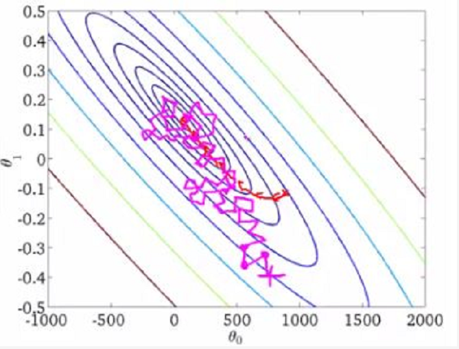
The comparison of batch gradient descent and random gradient descent on the three-dimensional graph is as follows:

The implementation of Python 3 based on gradient descent algorithm is as follows: (the annotation part is the implementation of BGD)

# -*- coding: cp936 -*-
import numpy as np
from scipy import stats
import matplotlib.pyplot as plt


# Construct training data
x = np.arange(0., 10., 0.2)
m = len(x)                                      # Number of training data points
x0 = np.full(m, 1.0)
input_data = np.vstack([x0, x]).T               # Take bias b as the first component of the weight vector
target_data = 2 * x + 5 + np.random.randn(m)


# Two termination conditions
loop_max = 10000   # Maximum number of iterations (prevent dead cycle)
epsilon = 1e-3

# Initialization weight
np.random.seed(0)
w = np.random.randn(2)
#w = np.zeros(2)

alpha = 0.001      # Step size (note that too large value leads to oscillation and too small convergence speed slows down)
diff = 0.
error = np.zeros(2)
count = 0          # Number of cycles
finish = 0         # Stop sign
# -------------------------------------------Random gradient descent algorithm----------------------------------------------------------

while count < loop_max:
    count += 1

    # Traverse the training data set and update the weights continuously
    for i in range(m):
        diff = np.dot(w, input_data[i]) - target_data[i]  # Substituting training set to calculate error value

        # Using random gradient descent algorithm, only one set of training data is used to update the weight once
        w = w - alpha * diff * input_data[i]

        # ------------------------------Judgment of termination conditions-----------------------------------------
        # If it is not terminated, continue to read the samples for processing. If all samples have been read, the loop will read the samples again from the beginning for processing.

    # ----------------------------------Judgment of termination conditions-----------------------------------------
    # Note: there are a variety of iteration termination conditions, and the location of the judgment statement. The termination judgment can be placed after the weight vector is updated once or m times.
    if np.linalg.norm(w - error) < epsilon:     # Termination condition: the absolute error of the weight vector calculated twice before and after is sufficiently small
        finish = 1
        break
    else:
        error = w
print ('loop count = %d' % count,  '\tw:[%f, %f]' % (w[0], w[1]))


# -----------------------------------------------Gradient descent method-----------------------------------------------------------


while count < loop_max:
    count += 1

    # The standard gradient descent is to sum up the errors of all samples before updating the weights, while the weights of random gradient descent are updated by examining a training sample
    # In standard gradient descent, more calculation is needed to sum multiple samples at each step of weight updating
    sum_m = np.zeros(2)
    for i in range(m):
        dif = (np.dot(w, input_data[i]) - target_data[i]) * input_data[i]
        sum_m = sum_m + dif     # When the alpha value is too large, sum_m will overflow during the iteration

    w = w - alpha * sum_m       # Pay attention to the value of step length alpha, which leads to oscillation
    #w = w - 0.005 * sum_m      # When the alpha is 0.005, the oscillation will occur, and the alpha needs to be reduced

    # Judge whether it has converged
    if np.linalg.norm(w - error) < epsilon:
        finish = 1
        break
    else:
        error = w
        
print ('loop count = %d' % count,  '\tw:[%f, %f]' % (w[0], w[1]))



# check with scipy linear regression
slope, intercept, r_value, p_value, slope_std_error = stats.linregress(x, target_data)
print ('intercept = %s slope = %s' %(intercept, slope))

plt.plot(x, target_data, 'k+')
plt.plot(x, w[1] * x + w[0], 'r')
plt.show()

[failed to transfer the pictures in the external link. The source station may have anti-theft chain mechanism. It is recommended to save the pictures and upload them directly (img-s0biasjK-1592112372128)(D:\CSDN\Blog92103434656.png))

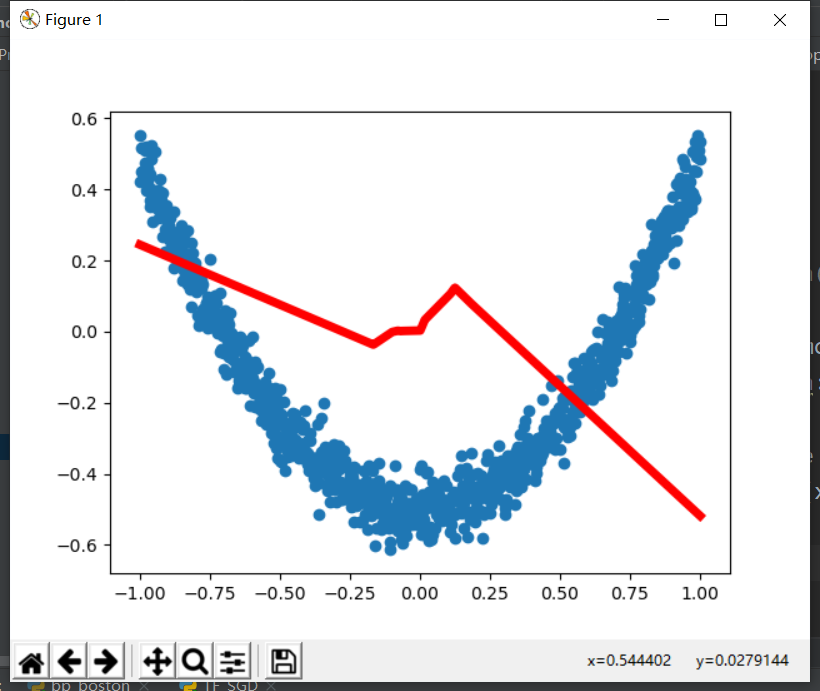
Random gradient descent visualization:

tensorflow 1.14 implementation:

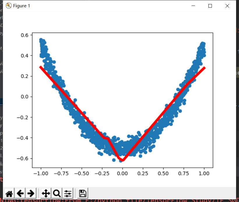
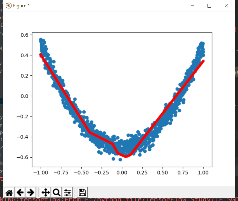
import tensorflow as tf
import numpy as np
import matplotlib.pyplot as plt


# Add layer
def add_layer(inputs, in_size, out_size, activation_function=None):
    W = tf.Variable(tf.random_normal([in_size, out_size]))
    b = tf.Variable(tf.zeros([1, out_size]) + 0.1)
    Wx_plus_b = tf.matmul(inputs, W) + b
    if activation_function is None:
        outputs = Wx_plus_b
    else:
        outputs = activation_function(Wx_plus_b)
    return outputs


# Generate input data, noise and output data
x_data = np.linspace(-1, 1, 1000)[:, np.newaxis]
noise = np.random.normal(0, 0.05, x_data.shape)
y_data = np.square(x_data) - 0.5 + noise

xs = tf.placeholder(tf.float32, [None, 1])
ys = tf.placeholder(tf.float32, [None, 1])

# Hidden and output layers
l1 = add_layer(xs, 1, 10, activation_function=tf.nn.relu)
prediction = add_layer(l1, 10, 1, activation_function=None)

# magnitude of the loss
loss = tf.reduce_mean(tf.reduce_sum(tf.square(ys - prediction),
                                    reduction_indices=[1]))

# Update loss with gradient descent
train_step = tf.train.GradientDescentOptimizer(0.1).minimize(loss)

# Initialize all parameters
init = tf.initialize_all_variables()
sess = tf.Session()
sess.run(init)

figure = plt.figure()
ax = figure.add_subplot(1, 1, 1)
ax.scatter(x_data, y_data)
plt.ion()
plt.show()


# 1000 workouts
for i in range(1000):
    sess.run(train_step, feed_dict={xs: x_data, ys: y_data})
    if i % 50 == 0:
        # print(sess.run(loss, feed_dict={xs: x_data, ys: y_data}))
        try:
            ax.lines.remove(lines[0])
        except Exception:
            pass
        prediction_value = sess.run(prediction, feed_dict={xs: x_data, ys: y_data})
        lines = ax.plot(x_data, prediction_value, 'r-', lw=5)

        plt.pause(0.1)

Results:

reference;https://www.cnblogs.com/itmorn/p/11129806.html