1, An overview of gradient descent algorithm
1, introduction
gradient descent, also known as the steepest descent, is the most commonly used method to solve unconstrained optimization problems. It is an iterative method. The main operation of each step is to solve the gradient vector of the objective function, taking the negative gradient direction of the current position as the search direction (because in this direction, the objective function declines the fastest, which is also the fastest The origin of the name of descending method).
Characteristics of gradient descent method: the closer to the target value, the smaller the step size and the slower the descent speed.
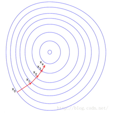
Here, each circle represents a function gradient, and the center represents the extreme point of the function. Each iteration finds a new position according to the gradient (used to determine the search direction and determine the forward speed together with the step size) and the step size obtained from the current position. In this way, the iteration continues until the local optimum of the objective function is achieved (if the objective function is convex, the global optimum is reached) .
We can more intuitively and clearly explain that gradient descent is actually a formula:
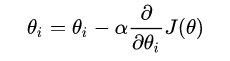
The above formula updates the formula. To put it bluntly, every step you take, you record your current position, that is, theta i to the left of the equal sign. How far is your step? The answer should be α. Which direction do you want to go? The answer is the partial derivative of J(θ) with respect to θ i.
Explain:
Here we distinguish the functions that are often used:
-
Loss Function is defined on a single sample, and it calculates the error of a sample.
-
Cost Function is defined in the whole training set, which is the average of all sample errors, that is, the average of loss function.
-
The Object Function is defined as the final function to be optimized. Equal to empirical risk + structural risk (that is, Cost Function + regularization term).
The J(θ) used in gradient descent is the loss function.
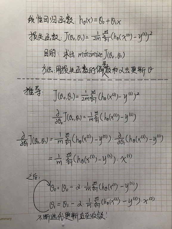
2. Deduction
Explain:
-
Here we use the linear regression function with two simple parameters θ 0 and θ 1 as an example to derive.
-
Knowledge used in derivation: partial derivative
3. A variety of gradient descent algorithm
There are three main variations of gradient descent algorithm, the main difference is how much data is used to calculate the gradient of the objective function. Different methods mainly make trade-offs between accuracy and optimization speed.
1.Batch gradient descent (BGD)
Batch gradient descent algorithm (BGD), which needs to calculate the gradient of the whole training set, namely:
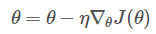
Where η is the learning rate, which is used to control the update "strength" / "step size".
- Advantage:
For convex objective function, the global optimization can be guaranteed; for non convex objective function, the local optimization can be guaranteed.
- Disadvantages:
Slow speed; infeasible with large amount of data; unable to optimize online (i.e. unable to process new samples generated dynamically).
2.Stochastic gradient descent (SGD)
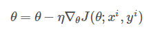
The random gradient descent algorithm (SGD) only calculates the gradient of a sample, i.e. updates the parameters for a training sample xi and its label yi:
Gradually reduce the learning rate, SGD performance is very similar to BGD, and finally can have good convergence.
- Advantage:
Fast update frequency, faster optimization speed; online optimization (can not deal with dynamically generated new samples); certain randomness leads to the probability of jumping out of local optimization (randomness comes from replacing the gradient of the whole sample with the gradient of one sample).
- Disadvantages:
Randomness may lead to the complexity of convergence, even if the best point is reached, it will be over optimized, so the optimization process of SGD is full of turbulence compared with BGD.
3.Mini-batch gradient descent (MBGD)
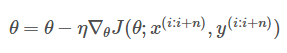
A small batch gradient descent algorithm (MBGD) is used to calculate the gradient of mini batch with n samples
MBGD is the most commonly used optimization method for training neural networks.
- Advantage:
When the parameters are updated, the turbulence becomes smaller, the convergence process is more stable, and the difficulty of convergence is reduced.
4, challenges
From the point of view of the < U > gradient descent algorithm varieties, < U > the mini batch gradient descent (MBGD) is a relatively good strategy, but it also can not guarantee an optimal solution. In addition, there are many problems to be solved:
1) How to choose the right learning rate?
Too small learning rate leads to too slow convergence, too large leads to convergence turbulence and even deviates from the best.
2) How to determine the adjustment strategy of learning rate?
At present, the adjustment learning rate basically adjusts according to the idea of "annealing" or adjusts according to the predetermined mode, or dynamically changes the learning rate according to whether the change of the objective function value meets the threshold. However, both mode and threshold need to be specified in advance and cannot adapt to different data sets.
3) Is it appropriate to use the same learning rate for all parameter updates?
If the data is sparse and the distribution of features is uneven, it seems that we should give a big update to the features that appear less.
4) How to jump out of local optimum?
In theory, only a strict convex function can obtain the global optimal solution through gradient descent. However, the neural network is basically faced with non convex objective functions, which means that the optimization is easy to fall into local optimization. In fact, our difficulties often come from "saddle points" rather than local minima. The same loss function value is usually found around the saddle point, which makes SGD difficult to work because the gradient in each direction is close to 0
5. Gradient descent optimization algorithm
Here are some gradient descent optimization methods commonly used in deep learning to solve the above problems. Some infeasible methods for high dimensional data, such as Newton's method in the second-order method, are no longer discussed.
-
Momentum
-
Nesterov accelerated gradient
-
Adagrad
-
Adadelta
-
RMSprop
-
Adam
-
AdaMax
All the above optimization algorithms, because the blogger's research is not in-depth, interested can go to Summary of gradient descent optimization algorithm Learn in detail.
2, Code practice
1. Batch gradient descent (BGD)
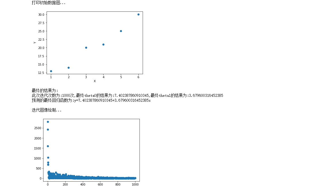
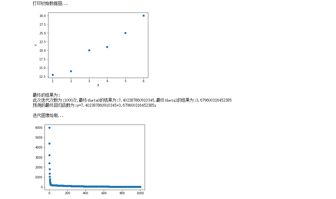
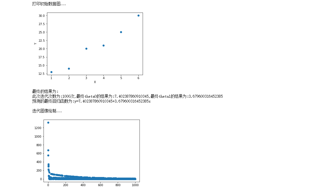
#Approach Library
#Introducing matplotlib library for drawing
import matplotlib.pyplot as plt
from math import pow
#Picture embedding jupyter
%matplotlib inline

#For the convenience of data access, we divide the data into x,y, which is the point in the rectangular coordinate system
x = [1,2,3,4,5,6]
y = [13,14,20,21,25,30]
print("Print initial data map...")
plt.scatter(x,y)
plt.xlabel("X")
plt.ylabel("Y")
plt.show()

#Super parameter setting
alpha = 0.01#Learning rate / step
theta0 = 0#θ0
theta1 = 0#θ1
epsilon = 0.001#error
m = len(x)

count = 0
loss = []

for time in range(1000):
    count += 1
    #The results of partial derivation theta 0 and theta 1
    temp0 = 0#The result of derivative of J(θ) to θ 0
    temp1 = 0#The result of derivative of J(θ) to θ 1
    diss = 0
    for i in range(m):
        temp0 += (theta0+theta1*x[i]-y[i])/m
        temp1 += ((theta0+theta1*x[i]-y[i])/m)*x[i]

    #Update theta0 and theta1
    for i in range(m):
        theta0 = theta0 - alpha*((theta0+theta1*x[i]-y[i])/m)
        theta1 = theta1 - alpha*((theta0+theta1*x[i]-y[i])/m)*x[i]

    #Find loss function J(θ)
    for i in range(m):
        diss = diss + 0.5*(1/m)*pow((theta0+theta1*x[i]-y[i]),2)
    loss.append(diss)

    #See if the conditions are met
    '''
    if diss<=epsilon:
        break
    else:
        continue
    '''
print("The final result is:")
print("The number of iterations is:{}second,Final theta0 The result is:{},Final theta1 The result is:{}".format(count,theta0,theta1))
print("The final regression function of the prediction is:y={}+{}x\n".format(theta0,theta1))
print("Iterative image rendering...")
plt.scatter(range(count),loss)
plt.show()
2. Random gradient descent (SGD)
#Approach Library
#Introducing matplotlib library for drawing
import matplotlib.pyplot as plt
from math import pow
import numpy as np
#Picture embedding jupyter
%matplotlib inline

#For the convenience of data access, we divide the data into x,y, which is the point in the rectangular coordinate system
x = [1,2,3,4,5,6]
y = [13,14,20,21,25,30]
print("Print initial data map...")
plt.scatter(x,y)
plt.xlabel("X")
plt.ylabel("Y")
plt.show()

#Super parameter setting
alpha = 0.01#Learning rate / step
theta0 = 0#θ0
theta1 = 0#θ1
epsilon = 0.001#error
m = len(x)

count = 0
loss = []

for time in range(1000):
    count += 1
    diss = 0
    #The results of partial derivation theta 0 and theta 1
    temp0 = 0#The result of derivative of J(θ) to θ 0
    temp1 = 0#The result of derivative of J(θ) to θ 1
    for i in range(m):
        temp0 += (theta0+theta1*x[i]-y[i])/m
        temp1 += ((theta0+theta1*x[i]-y[i])/m)*x[i]

    #Update theta0 and theta1
    for i in range(m):
        theta0 = theta0 - alpha*((theta0+theta1*x[i]-y[i])/m)
        theta1 = theta1 - alpha*((theta0+theta1*x[i]-y[i])/m)*x[i]

    #Find loss function J(θ)
    rand_i = np.random.randint(0,m)
    diss += 0.5*(1/m)*pow((theta0+theta1*x[rand_i]-y[rand_i]),2)
    loss.append(diss)

    #See if the conditions are met
    '''
    if diss<=epsilon:
        break
    else:
        continue
    '''
print("The final result is:")
print("The number of iterations is:{}second,Final theta0 The result is:{},Final theta1 The result is:{}".format(count,theta0,theta1))
print("The final regression function of the prediction is:y={}+{}x\n".format(theta0,theta1))
print("Iterative image rendering...")
plt.scatter(range(count),loss)
plt.show()
3. Small batch gradient descent (MBGD)
#Approach Library
#Introducing matplotlib library for drawing
import matplotlib.pyplot as plt
from math import pow
import numpy as np
#Picture embedding jupyter
%matplotlib inline

#For the convenience of data access, we divide the data into x,y, which is the point in the rectangular coordinate system
x = [1,2,3,4,5,6]
y = [13,14,20,21,25,30]
print("Print initial data map...")
plt.scatter(x,y)
plt.xlabel("X")
plt.ylabel("Y")
plt.show()

#Super parameter setting
alpha = 0.01#Learning rate / step
theta0 = 0#θ0
theta1 = 0#θ1
epsilon = 0.001#error
diss = 0#loss function
m = len(x)

count = 0
loss = []

for time in range(1000):
    count += 1
    diss = 0
    #The results of partial derivation theta 0 and theta 1
    temp0 = 0#The result of derivative of J(θ) to θ 0
    temp1 = 0#The result of derivative of J(θ) to θ 1
    for i in range(m):
        temp0 += (theta0+theta1*x[i]-y[i])/m
        temp1 += ((theta0+theta1*x[i]-y[i])/m)*x[i]

    #Update theta0 and theta1
    for i in range(m):
        theta0 = theta0 - alpha*((theta0+theta1*x[i]-y[i])/m)
        theta1 = theta1 - alpha*((theta0+theta1*x[i]-y[i])/m)*x[i]

    #Find loss function J(θ)
    result = []
    for i in range(3):
        rand_i = np.random.randint(0,m)
        result.append(rand_i)
    for j in result:
        diss += 0.5*(1/m)*pow((theta0+theta1*x[j]-y[j]),2)
    loss.append(diss)

    #See if the conditions are met
    '''
    if diss<=epsilon:
        break
    else:
        continue
    '''
print("The final result is:")
print("The number of iterations is:{}second,Final theta0 The result is:{},Final theta1 The result is:{}".format(count,theta0,theta1))
print("The final regression function of the prediction is:y={}+{}x\n".format(theta0,theta1))
print("Iterative image rendering...")
plt.scatter(range(count),loss)
plt.show()