date: 2020-01-11 15:51:39
Some time ago, my tutor asked me to know about the GreenPlum database. Later, I installed and used it for a while. It felt like it was no different from other databases, so it ended up. Now go over the features of GPDB and try to use them.
In fact, I really need to understand the characteristics written on the official propaganda page.
Characteristic
First of all, what are the features of GPDB? Where to find it? There must be on the product's leaflet.
Maximum characteristics
The biggest feature of GPDB is MPP, that is, Massively Parallel Processing. stay home page The most obvious are these two:
- Massively Parallel
- Analytics, analytics

Then, slide down the page, two obvious features are:
- Power at scale: high performance on petabyte scale data volumes.
- True Flexibility: Deploy anywhere. Deploy flexibly.


Main characteristics
The homepage then slides down, indicating the main features of GPDB:
- MPP Architecture
- Petabyte scale loading: the loading speed increases with the increase of each additional node, and the loading speed of each rack exceeds 10Tb/h (about 347.22 GB/s).
- Innovative Query Optimization: the first cost based query optimizer for big data workload in the industry
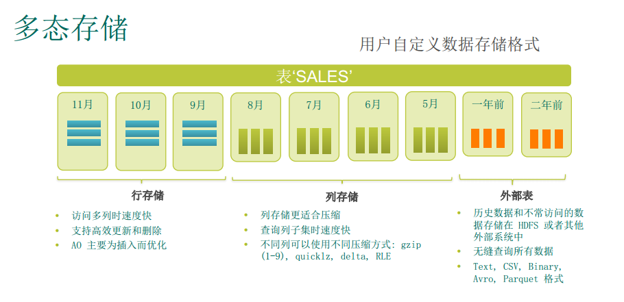
- Polymorphic Data Storage: Polymorphic Data Storage. Full control table and * – * * partitioned storage, execution, and compression configurations.
- Integrated in database Analytics: a library provided by Apache MADlib, which is used for analysis in scalable database. It extends the SQL function of Greenplum database through user-defined functions.
- Federated Data Access: Federated Data Access. Use Greenplum optimizer and query processing engine to query external data sources. Including Hadoop, Cloud Storage, ORC, AVRO, Parquet and other Polygot data storage.

Unfortunately, none of these icons on the home page can be clicked. So to experience these characteristics, we have to explore it by ourselves.
TODO
- Query data from hadoop.
GPDB vs. Hadoop + Hive
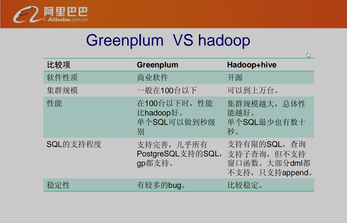
Source: Greenplum introduction , this is the report made by Alibaba on February 17, 2011. The GPDB version is 4.x
Compared with Hadoop + Hive, the query performance of GPDB is better than Hive, but the number of cluster nodes supported by GPDB is too small, up to 1000 segment s, and Hive can support tens of thousands of nodes.
Data Loading
There are mainly 3 loading methods:
- the SQL INSERT statement: inefficient when loading large amounts of data, suitable for small datasets.
- the COPY command: you can customize the format of the text file to parse into columns and rows. Faster than INSERT, but not a parallel process
-
gpfdist and gpload: can efficiently dump external data to the data table. Fast, parallel loading. The Administrator can define a single row error isolation mode to continue loading rows in a normal format. Gpload needs to write a yaml formed control file in advance to describe source data location,format, transformations required, participating hosts, database destinations, and others. This allows you to perform a complex loading task.
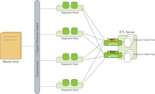
The following only demonstrates the use of gpfdist and gpload:
gpfdist
gpfdist [-d directory] [-p http_port] [-l log_file] [-t timeout]
   [-S] [-w time] [-v | -V] [-s] [-m max_length]
   [--ssl certificate_path [--sslclean wait_time] ]
   [-c config.yml]
Uses the gpfdist protocol to create a readable external table, ext_expenses, from all files with the txt extension. The column delimiter is a pipe(|) and NULL (' ') is a space. Access to the external table is single row error isolation mode. If the error count on a segment is greater than five (the SEGMENT REJECT LIMIT value), the entire external table operation fails and no rows are processed.
=# CREATE EXTERNAL TABLE ext_expenses ( name text,
   date date, amount float4, category text, desc1 text )
   LOCATION ('gpfdist://etlhost-1:8081/*.txt',
             'gpfdist://etlhost-2:8082/*.txt')
   FORMAT 'TEXT' ( DELIMITER '|' NULL ' ')
   LOG ERRORS SEGMENT REJECT LIMIT 5;
To create the readable ext_expenses table from CSV-formatted text files:
=# CREATE EXTERNAL TABLE ext_expenses ( name text,
   date date,  amount float4, category text, desc1 text )
   LOCATION ('gpfdist://etlhost-1:8081/*.txt',
             'gpfdist://etlhost-2:8082/*.txt')
   FORMAT 'CSV' ( DELIMITER ',' )
   LOG ERRORS SEGMENT REJECT LIMIT 5;
Here is my personal experiment:
-
Create a data directory ~ / Datasets/baike, and move the data set baike_triple.txt to this directory.
The dataset here comes from CN-DBpedia , containing 9 million + encyclopedia entities and 67 million + triple relationships. Among them, mention2entity information is 1.1 million +, summary information is 4 million +, label information is 19.8 million +, infobox information is 41 million +. The size is about 4.0 G. Data examples are as follows:
"1 + 8" Times Square
 "1 + 8" Times Square location Xianning Avenue and Yinquan Avenue intersection
 "1 + 8" times square real city complex project
 The total construction area of "1 + 8" Times Square is about 112800 square meters
 "1.4" fire accident in Lankao, Henan
 "1.4" fire accident location in Lankao County, Henan Province
 "1.4" Henan Lankao fire accident time: January 4, 2013
-
Open gpfdist background:
gpfdist -d ~/Datasets/baike -p 8081 > /tmp/gpfdist.log 2>&1 &
ps -A | grep gpfdist # View process number
30693 pts/8    00:00:00 gpfdist  # Indicates the process number is 30693
Option Description:
- -d directory: specifies a directory from which gpfdist will provide files for readable external tables or create output files for writable external tables. If not specified, defaults to the current directory.
- -P http_port: gpfdist provides the HTTP port to use for files. The default is 8080.
View log:
gt@vm1:~$ more /tmp/gpfdist.log
2020-01-13 02:49:38 30693 INFO Before opening listening sockets - following listening sockets are a vailable:
2020-01-13 02:49:38 30693 INFO IPV6 socket: [::]:8081
2020-01-13 02:49:38 30693 INFO IPV4 socket: 0.0.0.0:8081
2020-01-13 02:49:38 30693 INFO Trying to open listening socket:
2020-01-13 02:49:38 30693 INFO IPV6 socket: [::]:8081
2020-01-13 02:49:38 30693 INFO Opening listening socket succeeded
2020-01-13 02:49:38 30693 INFO Trying to open listening socket:
2020-01-13 02:49:38 30693 INFO IPV4 socket: 0.0.0.0:8081
Serving HTTP on port 8081, directory /home/gt/Datasets/baike
-
Open a psql session as gpadmin, and create tables: ext Baike to store the loaded data, and ext load Baike err to store the loading error log.
psql -h localhost -d db_kg # Enter DB? Kg

# Create external table
CREATE EXTERNAL TABLE ext_baike (
head text, rel text, tail text)
LOCATION ('gpfdist://vm1:8081/baike_triples.txt')
FORMAT 'TEXT' (DELIMITER E'\t')
LOG ERRORS SEGMENT REJECT LIMIT 50000;

# Create internal storage table
CREATE TABLE tb_baike (
id SERIAL PRIMARY KEY, head text, rel text, tail text);
Create external table syntax details: CREATE EXTERNAL TABLE .
After creating an external table, you can read data directly from the external table, for example:
db_kg=# select * from ext_baike limit 10;
      head       |   rel    |     tail
-----------------+----------+---------------
 *Descent*            | Chinese name   | *Descent*
 *Descent*            | author     | Amarantine
 *Descent*            | Fiction progress | suspend
 *Descent*            | Serialized website | Jinjiang literature City
 *Introduction to western criminology | BaiduTAG | book
 *Introduction to western criminology | ISBN     | 9787811399967
 *Introduction to western criminology | author     | Edited by Li Mingqi
 *Introduction to western criminology | Publishing time | 2010-4
 *Introduction to western criminology | Price     | 22.00element
 *Introduction to western criminology | The number of pages     | 305
(10 rows)
-
To import external table data into an internal table:
INSERT INTO tb_baike(head, rel, tail) SELECT * FROM ext_baike;
The last run failed due to insufficient storage space for the virtual machine. You can see in the log:
more greenplum/data/data1/primary/gpseg0/pg_log/gpdb-2020-01-13_000000.csv
2020-01-13 04:10:14.623480 UTC,,,p24832,th930718592,,,,0,,,seg0,,,,,"PANIC","53100","could not writ
e to file ""pg_xlog/xlogtemp.24832"": No space left on device",,,,,,,0,,"xlog.c"
start: 15:33:30
abnormally end: 16:03
Error:
db_kg=# INSERT INTO tb_baike(head, rel, tail) SELECT * FROM ext_baike;
ERROR: gpfdist error: unknown meta type 108 (url_curl.c:1635) (seg0 slice1 127.0.1.1:6000 pid=15880) (url_curl.c:1635)
CONTEXT: External table ext_baike, file gpfdist://vm1:8081/baike_triples.txtLIMIT 10000;
start 16:10:00
end: 17:12:42
ERROR: interconnect encountered a network error, please check your network (seg3 slice1 192.168.5
6.6:6001 pid=11612)
DETAIL: Failed to send packet (seq 1) to 127.0.1.1:56414 (pid 15913 cid -1) after 3562 retries in
3600 seconds
Cost-based Query Optimizer
When the master receives an SQL statement, it will parse the statement into an execution plan DAG. When the DAG is divided into slice, join, aggregate and sort, which do not need data exchange, the redistribution of slice will be involved. There will be a motion task to perform data redistribution. Distribute slice to the relevant segment s involved. Source: GreenPlum: distributed relational database based on PostgreSQL
Reference resources About Greenplum Query Processing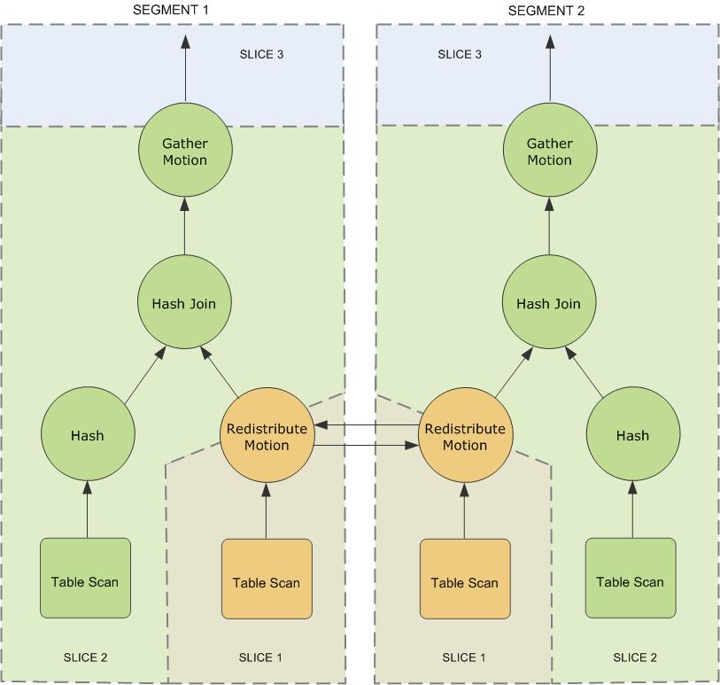
slice: To achieve maximum parallelism during query execution, Greenplum divides the work of the query plan into slices. A slice is a portion of the plan that segments can work on independently. A query plan is sliced wherever a motion operation occurs in the plan, with one slice on each side of the motion.
motion: A motion operation involves moving tuples between the segments during query processing. Note that not every query requires a motion. For example, a targeted query plan does not require data to move across the interconnect.
- a redistribute motion that moves tuples between the segments to complete the join.
- A gather motion is when the segments send results back up to the master for presentation to the client. Because a query plan is always sliced wherever a motion occurs, this plan also has an implicit slice at the very top of the plan (slice 3).
Federated Data Access
MADlib extension
Add madlib extension
from Pivotal Network Download MADlib 1.16+8 for RHEL 7
To install using gppkg:
An error occurred:
gt@vm1:~/madlib-1.16+8-gp6-rhel7-x86_64$ gppkg -i madlib-1.16+8-gp6-rhel7-x86_64.gppkg
20200113:10:01:15:018921 gppkg:vm1:gt-[INFO]:-Starting gppkg with args: -i madlib-1.16+8-gp6-rhel7-x86_64.gppkg
20200113:10:01:15:018921 gppkg:vm1:gt-[CRITICAL]:-gppkg failed. (Reason='__init__() takes exactly 17 arguments (16 given)') exiting...
Finally, the system is reinstalled: Centos 7 Pivotal Network The following describes the systems that madlib can install: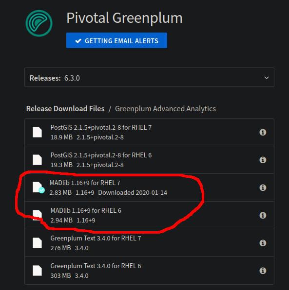
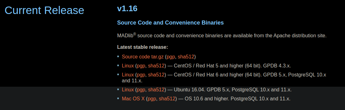
The Pivotal Network only provides the binary package of Redhat 6.x and Redhat 7.x. Ubuntu 18.04 installed before cannot be used. We can't use Redhat Enterprise Linux.. So consider using a free Fedora or CentOS system. I installed CentOS 7,
[gpadmin@vm1 ~]$ cat /etc/os-release
NAME="CentOS Linux"
VERSION="7 (Core)"
ID="centos"
ID_LIKE="rhel fedora"
VERSION_ID="7"
PRETTY_NAME="CentOS Linux 7 (Core)"
ANSI_COLOR="0;31"
CPE_NAME="cpe:/o:centos:centos:7"
HOME_URL="https://www.centos.org/"
BUG_REPORT_URL="https://bugs.centos.org/"

CENTOS_MANTISBT_PROJECT="CentOS-7"
CENTOS_MANTISBT_PROJECT_VERSION="7"
REDHAT_SUPPORT_PRODUCT="centos"
REDHAT_SUPPORT_PRODUCT_VERSION="7"
The Greenplum installed is version 6.3. Therefore, the downloaded file is madlib-1.16 + 9-gp6-rhel7-x86_.tar.gz. After decompression, it is as follows:
[gpadmin@vm1 madlib-1.16+9-gp6-rhel7-x86_64]$ ls -la
total 3048
drwxr-xr-x. 2 gpadmin gpadmin     147 Jan 14 16:51 .
drwx------. 7 gpadmin gpadmin    4096 Jan 14 16:51 ..
-rw-r--r--. 1 gpadmin gpadmin 2904455 Jan 10 07:31 madlib-1.16+9-gp6-rhel7-x86_64.gppkg
-rw-r--r--. 1 gpadmin gpadmin  135530 Jan 10 07:31 open_source_license_MADlib_1.16_GA.txt
-rw-r--r--. 1 gpadmin gpadmin   61836 Jan 10 07:31 ReleaseNotes.txt
The file of madlib-1.16 + 9-gp6-rhel7-x86_.gppkg in it needs to be installed using the gppkg tool of GreenPlum. The installation method is:
${GPHOME}/bin/gppgk [-i <package>| -u <package> | -r <name-version> | -c]
[-d <master_data_directory>] [-a] [-v]
Installation:
${GPHOME}/bin/gppgk -i madlib-1.16+9-gp6-rhel7-x86_64.gppkg
Then, install MADlib Object to Database:
$GPHOME/madlib/bin/madpack install -s madlib -p greenplum -c gpadmin@vm1:5432/testdb
The installation records are as follows (M4 and Yum install M4 need to be installed in advance):
[gpadmin@vm1 madlib-1.16+9-gp6-rhel7-x86_64]$ $GPHOME/madlib/bin/madpack install -p greenplum
madpack.py: INFO : Detected Greenplum DB version 6.3.0.
madpack.py: INFO : *** Installing MADlib ***
madpack.py: INFO : MADlib tools version    = 1.16 (/usr/local/greenplum-db-6.3.0/madlib/Versions/1.16/bin/../madpack/madpack.py)
madpack.py: INFO : MADlib database version = None (host=localhost:5432, db=gpadmin, schema=madlib)
madpack.py: INFO : Testing PL/Python environment...
madpack.py: INFO : > PL/Python environment OK (version: 2.7.12)
madpack.py: INFO : > Preparing objects for the following modules:
madpack.py: INFO : > - array_ops
madpack.py: INFO : > - bayes
madpack.py: INFO : > - crf
madpack.py: INFO : > - elastic_net
madpack.py: INFO : > - linalg
madpack.py: INFO : > - pmml
madpack.py: INFO : > - prob
madpack.py: INFO : > - sketch
madpack.py: INFO : > - svec
madpack.py: INFO : > - svm
madpack.py: INFO : > - tsa
madpack.py: INFO : > - stemmer
madpack.py: INFO : > - conjugate_gradient
madpack.py: INFO : > - knn
madpack.py: INFO : > - lda
madpack.py: INFO : > - stats
madpack.py: INFO : > - svec_util
madpack.py: INFO : > - utilities
madpack.py: INFO : > - assoc_rules
madpack.py: INFO : > - convex
madpack.py: INFO : > - deep_learning
madpack.py: INFO : > - glm
madpack.py: INFO : > - graph
madpack.py: INFO : > - linear_systems
madpack.py: INFO : > - recursive_partitioning
madpack.py: INFO : > - regress
madpack.py: INFO : > - sample
madpack.py: INFO : > - summary
madpack.py: INFO : > - kmeans
madpack.py: INFO : > - pca
madpack.py: INFO : > - validation
madpack.py: INFO : Installing MADlib:
madpack.py: INFO : > Created madlib schema
madpack.py: INFO : > Created madlib.MigrationHistory table
madpack.py: INFO : > Wrote version info in MigrationHistory table
madpack.py: INFO : MADlib 1.16 installed successfully in madlib schema.
Use of madlib
Error (in DB? Kg):
ERROR: schema "madlib" does not exist
Since no database is specified when installing madlib with madpack, an error will occur when using madlib in DB? Kg. Use madpack install check to check:
[gpadmin@vm1 ~]$ $GPHOME/madlib/bin/madpack install-check -p greenplum -c gpadmin@vm1:5432/db_madlib_demo
madpack.py: INFO : Detected Greenplum DB version 6.3.0.
madpack.py: INFO : MADlib is not installed in the schema madlib. Install-check stopped.
It is found that madlib is not installed in the database db? Kg. Look at the log of madpack install above. It is found that the default database selected is gpadmin, that is, the database with the same user name:
madpack.py: INFO : MADlib database version = None (host=localhost:5432, db=gpadmin, schema=madlib)
Test on DB? Kg database and find that it has been installed:
[gpadmin@vm1 ~]$ $GPHOME/madlib/bin/madpack install-check -p greenplum
madpack.py: INFO : Detected Greenplum DB version 6.3.0.
TEST CASE RESULT|Module: array_ops|array_ops.ic.sql_in|PASS|Time: 203 milliseconds
TEST CASE RESULT|Module: bayes|bayes.ic.sql_in|PASS|Time: 1102 milliseconds
TEST CASE RESULT|Module: crf|crf_test_small.ic.sql_in|PASS|Time: 931 milliseconds
TEST CASE RESULT|Module: crf|crf_train_small.ic.sql_in|PASS|Time: 927 milliseconds
TEST CASE RESULT|Module: elastic_net|elastic_net.ic.sql_in|PASS|Time: 1041 milliseconds
TEST CASE RESULT|Module: linalg|linalg.ic.sql_in|PASS|Time: 274 milliseconds
TEST CASE RESULT|Module: linalg|matrix_ops.ic.sql_in|PASS|Time: 4158 milliseconds
TEST CASE RESULT|Module: linalg|svd.ic.sql_in|PASS|Time: 2050 milliseconds
TEST CASE RESULT|Module: pmml|pmml.ic.sql_in|PASS|Time: 2597 milliseconds
TEST CASE RESULT|Module: prob|prob.ic.sql_in|PASS|Time: 67 milliseconds
TEST CASE RESULT|Module: svm|svm.ic.sql_in|PASS|Time: 1479 milliseconds
TEST CASE RESULT|Module: tsa|arima.ic.sql_in|PASS|Time: 2058 milliseconds
TEST CASE RESULT|Module: stemmer|porter_stemmer.ic.sql_in|PASS|Time: 107 milliseconds
TEST CASE RESULT|Module: conjugate_gradient|conj_grad.ic.sql_in|PASS|Time: 555 milliseconds
TEST CASE RESULT|Module: knn|knn.ic.sql_in|PASS|Time: 574 milliseconds
TEST CASE RESULT|Module: lda|lda.ic.sql_in|PASS|Time: 641 milliseconds
TEST CASE RESULT|Module: stats|anova_test.ic.sql_in|PASS|Time: 147 milliseconds
TEST CASE RESULT|Module: stats|chi2_test.ic.sql_in|PASS|Time: 174 milliseconds
TEST CASE RESULT|Module: stats|correlation.ic.sql_in|PASS|Time: 426 milliseconds
TEST CASE RESULT|Module: stats|cox_prop_hazards.ic.sql_in|PASS|Time: 586 milliseconds
TEST CASE RESULT|Module: stats|f_test.ic.sql_in|PASS|Time: 129 milliseconds
TEST CASE RESULT|Module: stats|ks_test.ic.sql_in|PASS|Time: 138 milliseconds
TEST CASE RESULT|Module: stats|mw_test.ic.sql_in|PASS|Time: 118 milliseconds
TEST CASE RESULT|Module: stats|pred_metrics.ic.sql_in|PASS|Time: 779 milliseconds
TEST CASE RESULT|Module: stats|robust_and_clustered_variance_coxph.ic.sql_in|PASS|Time: 864 milliseconds
TEST CASE RESULT|Module: stats|t_test.ic.sql_in|PASS|Time: 145 milliseconds
TEST CASE RESULT|Module: stats|wsr_test.ic.sql_in|PASS|Time: 149 milliseconds
TEST CASE RESULT|Module: utilities|encode_categorical.ic.sql_in|PASS|Time: 425 milliseconds
TEST CASE RESULT|Module: utilities|minibatch_preprocessing.ic.sql_in|PASS|Time: 534 milliseconds
TEST CASE RESULT|Module: utilities|path.ic.sql_in|PASS|Time: 387 milliseconds
TEST CASE RESULT|Module: utilities|pivot.ic.sql_in|PASS|Time: 287 milliseconds
TEST CASE RESULT|Module: utilities|sessionize.ic.sql_in|PASS|Time: 245 milliseconds
TEST CASE RESULT|Module: utilities|text_utilities.ic.sql_in|PASS|Time: 334 milliseconds
TEST CASE RESULT|Module: utilities|transform_vec_cols.ic.sql_in|PASS|Time: 427 milliseconds
TEST CASE RESULT|Module: utilities|utilities.ic.sql_in|PASS|Time: 311 milliseconds
TEST CASE RESULT|Module: assoc_rules|assoc_rules.ic.sql_in|PASS|Time: 1328 milliseconds
TEST CASE RESULT|Module: convex|lmf.ic.sql_in|PASS|Time: 409 milliseconds
TEST CASE RESULT|Module: convex|mlp.ic.sql_in|PASS|Time: 2032 milliseconds
TEST CASE RESULT|Module: deep_learning|keras_model_arch_table.ic.sql_in|PASS|Time: 498 milliseconds
TEST CASE RESULT|Module: glm|glm.ic.sql_in|PASS|Time: 4514 milliseconds
TEST CASE RESULT|Module: graph|graph.ic.sql_in|PASS|Time: 4471 milliseconds
TEST CASE RESULT|Module: linear_systems|dense_linear_sytems.ic.sql_in|PASS|Time: 313 milliseconds
TEST CASE RESULT|Module: linear_systems|sparse_linear_sytems.ic.sql_in|PASS|Time: 376 milliseconds
TEST CASE RESULT|Module: recursive_partitioning|decision_tree.ic.sql_in|PASS|Time: 807 milliseconds
TEST CASE RESULT|Module: recursive_partitioning|random_forest.ic.sql_in|PASS|Time: 649 milliseconds
TEST CASE RESULT|Module: regress|clustered.ic.sql_in|PASS|Time: 549 milliseconds
TEST CASE RESULT|Module: regress|linear.ic.sql_in|PASS|Time: 104 milliseconds
TEST CASE RESULT|Module: regress|logistic.ic.sql_in|PASS|Time: 720 milliseconds
TEST CASE RESULT|Module: regress|marginal.ic.sql_in|PASS|Time: 1230 milliseconds
TEST CASE RESULT|Module: regress|multilogistic.ic.sql_in|PASS|Time: 1052 milliseconds
TEST CASE RESULT|Module: regress|robust.ic.sql_in|PASS|Time: 498 milliseconds
TEST CASE RESULT|Module: sample|balance_sample.ic.sql_in|PASS|Time: 389 milliseconds
TEST CASE RESULT|Module: sample|sample.ic.sql_in|PASS|Time: 79 milliseconds
TEST CASE RESULT|Module: sample|stratified_sample.ic.sql_in|PASS|Time: 252 milliseconds
TEST CASE RESULT|Module: sample|train_test_split.ic.sql_in|PASS|Time: 506 milliseconds
TEST CASE RESULT|Module: summary|summary.ic.sql_in|PASS|Time: 457 milliseconds
TEST CASE RESULT|Module: kmeans|kmeans.ic.sql_in|PASS|Time: 2581 milliseconds
TEST CASE RESULT|Module: pca|pca.ic.sql_in|PASS|Time: 4804 milliseconds
TEST CASE RESULT|Module: pca|pca_project.ic.sql_in|PASS|Time: 1948 milliseconds
TEST CASE RESULT|Module: validation|cross_validation.ic.sql_in|PASS|Time: 756 milliseconds
So install madlib on DB? Kg.
Check whether madlib is installed in the database:
[gpadmin@vm1 ~]$ psql -d db_madlib_demo
psql (9.4.24)
Type "help" for help.

db_madlib_demo=# \dn madlib
 List of schemas
  Name  |  Owner
--------+---------
 madlib | gpadmin
(1 row)
Body start
For the use of MADlib, please refer to: MADlib Documentation . too much content, just a few cases to learn.
Array Operations
Array Operations, copy from Array Operations:
| Operation | Description |
|---|---|
| array_add() | Adds two arrays. It requires that all the values are NON-NULL. Return type is the same as the input type. |
| sum() | Aggregate, sums vector element-wisely. It requires that all the values are NON-NULL. Return type is the same as the input type. |
| array_sub() | Subtracts two arrays. It requires that all the values are NON-NULL. Return type is the same as the input type. |
| array_mult() | Element-wise product of two arrays. It requires that all the values are NON-NULL. Return type is the same as the input type. |
| array_div() | Element-wise division of two arrays. It requires that all the values are NON-NULL. Return type is the same as the input type. |
| array_dot() | Dot-product of two arrays. It requires that all the values are NON-NULL. Return type is the same as the input type. |
| array_contains() | Checks whether one array contains the other. This function returns TRUE if each non-zero element in the right array equals to the element with the same index in the left array. |
| array_max() | This function finds the maximum value in the array. NULLs are ignored. Return type is the same as the input type. |
| array_max_index() | This function finds the maximum value and corresponding index in the array. NULLs are ignored. Return type is array in format [max, index], and its element type is the same as the input type. |
| array_min() | This function finds the minimum value in the array. NULLs are ignored. Return type is the same as the input type. |
| array_min_index() | This function finds the minimum value and corresponding index in the array. NULLs are ignored. Return type is array in format [min, index], and its element type is the same as the input type. |
| array_sum() | This function finds the sum of the values in the array. NULLs are ignored. Return type is the same as the input type. |
| array_sum_big() | This function finds the sum of the values in the array. NULLs are ignored. Return type is always FLOAT8 regardless of input. This function is meant to replace array_sum() in cases when a sum may overflow the element type. |
| array_abs_sum() | This function finds the sum of abs of the values in the array. NULLs are ignored. Return type is the same as the input type. |
| array_abs() | This function takes an array as the input and finds abs of each element in the array, returning the resulting array. It requires that all the values are NON-NULL. |
| array_mean() | This function finds the mean of the values in the array. NULLs are ignored. |
| array_stddev() | This function finds the standard deviation of the values in the array. NULLs are ignored. |
| array_of_float() | This function creates an array of set size (the argument value) of FLOAT8, initializing the values to 0.0. |
| array_of_bigint() | This function creates an array of set size (the argument value) of BIGINT, initializing the values to 0. |
| array_fill() | This functions set every value in the array to some desired value (provided as the argument). |
| array_filter() | This function takes an array as the input and keep only elements that satisfy the operator on specified scalar. It requires that the array is 1-D and all the values are NON-NULL. Return type is the same as the input type. By default, this function removes all zeros. |
| array_scalar_mult() | This function takes an array as the input and executes element-wise multiplication by the scalar provided as the second argument, returning the resulting array. It requires that all the values are NON-NULL. Return type is the same as the input type. |
| array_scalar_add() | This function takes an array as the input and executes element-wise addition of the scalar provided as the second argument, returning the resulting array. It requires that all the values are NON-NULL. Return type is the same as the input type. |
| array_sqrt() | This function takes an array as the input and finds square root of each element in the array, returning the resulting array. It requires that all the values are NON-NULL. |
| array_pow() | This function takes an array and a float8 as the input and finds power of each element in the array, returning the resulting array. It requires that all the values are NON-NULL. |
| array_square() | This function takes an array as the input and finds square of each element in the array, returning the resulting array. It requires that all the values are NON-NULL. |
| normalize() | This function normalizes an array as sum of squares to be 1. It requires that the array is 1-D and all the values are NON-NULL. |
| array_unnest_2d_to_1d() | This function takes a 2-D array as the input and unnests it by one level. It returns a set of 1-D arrays that correspond to rows of the input array as well as an ID column with values corresponding to row positions occupied by those 1-D arrays within the 2-D array. |
Example:
-
Create data table and insert data
CREATE TABLE array_tbl ( id integer NOT NULL PRIMARY KEY,
                         array1 integer[],
                         array2 integer[]
                       );
INSERT INTO array_tbl VALUES
                       ( 1, '{1,2,3,4,5,6,7,8,9}', '{9,8,7,6,5,4,3,2,1}' ),
                       ( 2, '{1,1,0,1,1,2,3,99,8}','{0,0,0,-5,4,1,1,7,6}' );
-
Using functions
db_madlib_demo=# select id,
						madlib.array_sum(array1),
						madlib.array_sub(array2, array1),
						madlib.array_max(array1),
						madlib.array_min(array1),
						madlib.array_mean(array1),
						madlib.normalize(array1)
				from array_tbl group by id;

 id | array_sum |          array_sub          | array_max | array_min |    array_mean    |
                         normalize
----+-----------+-----------------------------+-----------+-----------+------------------+-----------------------------------------------------
-----------------------------------------------------------------------------------------------------------------
  1 |        45 | {8,6,4,2,0,-2,-4,-6,-8}     |         9 |         1 |                5 | {0.0592348877759092,0.118469775551818,0.177704663327
728,0.236939551103637,0.296174438879546,0.355409326655455,0.414644214431365,0.473879102207274,0.533113989983183}
  2 |       116 | {-1,-1,0,-6,3,-1,-2,-92,-2} |        99 |         0 | 12.8888888888889 | {0.0100595273380576,0.0100595273380576,0,0.010059527
3380576,0.0100595273380576,0.0201190546761152,0.0301785820141728,0.995893206467704,0.0804762187044609}
(2 rows)
Low-Rank Matrix Faxtorization
This module uses a low rank approval to realize the decomposition of incomplete matrix.
Mathematically, this model seeks to find matrices U and V (also referred as factors) that, for any given incomplete matrix A, minimizes:
∣∣A−UVT∣∣2||A - UV^T||_2∣∣A−UVT∣∣2, s.t. rank(UVT)<=rrank(UV^T) <= rrank(UVT)<=r,
where ∣∣.∣∣2||.||_2∣∣.∣∣2 denotes the Frobenius norm. Let AAA be a m×nm×nm×n matrix, then UUU will be m×rm×rm×r and VVV will be n×rn×rn×r, in dimension, and 1≤r≪min(m,n)1≤r≪min(m,n)1≤r≪min(m,n). This model is not intended to do the full decomposition, or to be used as part of inverse procedure. This model has been widely used in recommendation systems (e.g., Netflix [2]) and feature selection (e.g., image processing [3]).
Function Syntax
lmf_igd_run( rel_output, # TEXT. The name of the table to receive the output.
             rel_source, # TEXT. The name of the table containing the input data.{sparse}
             col_row,	 # TEXT. The name of the column containing the row number.
             col_column, # TEXT. The name of the column containing the column number.
             col_value,	 # DOUBLE PRECISION. The value at (row, col).
             row_dim,	 # INTEGER, default: "SELECT max(col_row) FROM rel_source".
             column_dim, # INTEGER, default: "SELECT max(col_col) FROM rel_source".
             max_rank,	 # INTEGER, default: 20. The rank of desired approximation.
             stepsize,	 # DOUBLE PRECISION, default: 0.01. Hyper-parameter that decides how aggressive the gradient steps are.
             scale_factor, # DOUBLE PRECISION, default: 0.1. Hyper-parameter that decides scale of initial factors.
             num_iterations, # INTEGER, default: 10. Maximum number if iterations to perform regardless of convergence.
             tolerance # DOUBLE PRECISION, default: 0.0001. Acceptable level of error in convergence.
           )
Examples
-
Create table, insert data.
CREATE TABLE lmf_data (row INT, col INT, val FLOAT8, primary key (row, col));
INSERT INTO lmf_data VALUES (1, 1, 5.0), (3, 100, 1.0), (999, 10000, 2.0);
-
execute function
db_madlib_demo=# SELECT madlib.lmf_igd_run('lmf_model', 'lmf_data', 'row', 'col', 'val', 999,10000, 3, 0.1, 2, 10, 1e-9 );
NOTICE:  Matrix lmf_data to be factorized: 999 x 10000
NOTICE:  Table doesn't have 'DISTRIBUTED BY' clause -- Using column named 'id' as the Greenplum Database data distribution key for this table.
HINT:  The 'DISTRIBUTED BY' clause determines the distribution of data. Make sure column(s) chosen are the optimal data distribution key to minimize skew.
CONTEXT:  SQL statement "
            CREATE TABLE lmf_model (
                id          SERIAL,
                matrix_u    DOUBLE PRECISION[],
                matrix_v    DOUBLE PRECISION[],
                rmse        DOUBLE PRECISION)"
PL/pgSQL function madlib.lmf_igd_run(character varying,regclass,character varying,character varying,character varying,integer,integer,integer,double precision,double precision,integer,double precision) line 47 at EXECUTE statement
NOTICE:
Finished low-rank matrix factorization using incremental gradient
DETAIL:
 * table : lmf_data (row, col, val)
Results:
 * RMSE = 3.61661832699015e-06
Output:
 * view : SELECT * FROM lmf_model WHERE id = 1
 lmf_igd_run
-------------
           1
(1 row)
-
Check the result.
db_madlib_demo=# SELECT array_dims(matrix_u) AS u_dims, array_dims(matrix_v) AS v_dims
	FROM lmf_model
	WHERE id=1;

    u_dims    |     v_dims
--------------+----------------
 [1:999][1:3] | [1:10000][1:3]
(1 row)
-
Query the result value
db_madlib_demo=# SELECT matrix_u[2:2][1:3] AS row_2_features
	FROM lmf_model
	WHERE id = 1;

                     row_2_features
---------------------------------------------------------
 {{1.97037281095982,0.312463999725878,1.06016968935728}}
(1 row)
-
Make prediction of a missing entry (row=2, col=7654).
db_madlib_demo=# SELECT madlib.array_dot(
        matrix_u[2:2][1:3],
        matrix_v[7654:7654][1:3]
	) AS row_2_col_7654
		FROM lmf_model
		WHERE id = 1;

  row_2_col_7654
------------------
 2.37682774869935
(1 row)
Singular Value Decomposition
# SVD Function for Dense Matrices
svd( source_table, 			# TEXT. Source table name (dense matrix).
     output_table_prefix,	# TEXT. Prefix for output tables.
     row_id,				# TEXT. ID for each row.
     k,						# INTEGER. Number of singular values to compute.
     n_iterations,			# INTEGER. Number of iterations to run.
     result_summary_table	# TEXT. The name of the table to store the result summary.
);

# SVD Function for Sparse Matrices
svd_sparse( source_table,
    output_table_prefix,
    row_id,
    col_id,
    value,
    row_dim,
    col_dim,
    k,
    n_iterations,
    result_summary_table
    );
Neural Network
Classification Training Function
mlp_classification(
    source_table,
    output_table,
    independent_varname,
    dependent_varname,
    hidden_layer_sizes,
    optimizer_params,
    activation,
    weights,
    warm_start,
    verbose,
    grouping_col
    )
Regression Training Function
mlp_regression(
    source_table,
    output_table,
    independent_varname,
    dependent_varname,
    hidden_layer_sizes,
    optimizer_params,
    activation,
    weights,
    warm_start,
    verbose,
    grouping_col
    )
Optimizer Parameters
  'learning_rate_init = <value>,
   learning_rate_policy = <value>,
   gamma = <value>,
   power = <value>,
   iterations_per_step = <value>,
   n_iterations = <value>,
   n_tries = <value>,
   lambda = <value>,
   tolerance = <value>,
   batch_size = <value>,
   n_epochs = <value>,
   momentum = <value>,
   nesterov = <value>'
Prediction Function
mlp_predict(
    model_table,
    data_table,
    id_col_name,
    output_table,
    pred_type
    )
...
There are many other functions, there is no one-to-one experiment, you need to use it to find it.
In short, this thing, personal feeling is the edge of the database use case. The core feature of Greenplum is Analysis, but it's Apache. Is it a selling point.. Moreover, using database to analyze data, emmm, always feels a little inconsistent. In addition, Greenplum itself is not stable, and there are still many bug s. The previous load of massive data failed (gpfdist).
Of course, this tool is convenient. The data is processed in the place where the data is stored.
In a word, it's good to know that there is such a thing.

