Fundamentals of machine learning

The essence of machine learning: using data to solve problems

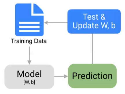
Data preprocessing (important in deep learning) - > training phase - > model generation - > prediction phase

We usually choose some data as the test set, such as about 20%.

Sometimes there is an additional verification set of about 20%

• Training phase: create a prediction model through data training and fine tune it.
• Model generation: the prediction model can find the answer behind these data and help us solve a problem.
• Prediction stage: complete the model evaluation through the test set, so as to understand the effectiveness of the model in the test set.

In this process, the prediction model will be continuously improved and used

Further, the steps of machine learning are as follows:

Data collection - > data preprocessing - > model selection - > Training - > evaluation - > superparameter adjustment - > prediction

loss function: an index to evaluate machine learning

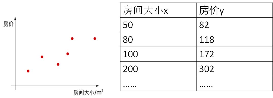
Example: forecast house prices

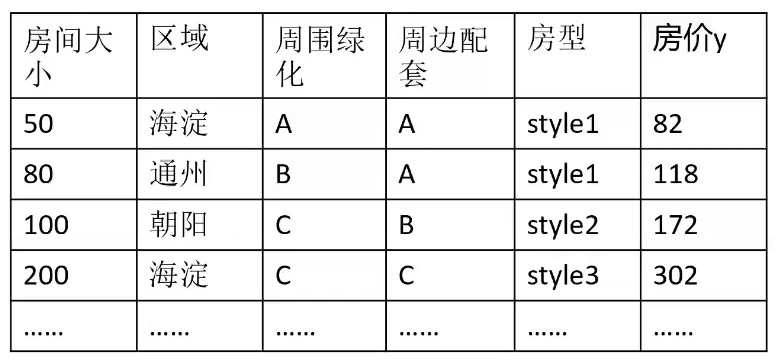
For features such as "region", it is necessary to discretize them by one hot coding, label coding, etc.

Tag encoding is often used to convert data elements of non numeric type [string, etc.)

For example, Haidian, Tongzhou and Chaoyang correspond to values 1, 2 and 3 respectively

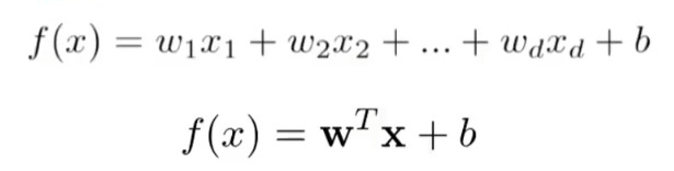
Machine learning often has many features. Based on these features, we need to train the weight w in the Model. The features composed of these eigenvalues are called weight matrix Weights, and there are biases.

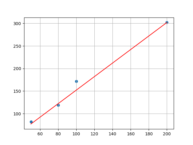
Using linear regression to predict house prices

Violent exhaustion:

import numpy as np
import matplotlib.pyplot as plt

#MAE loss function
def MAE_loss(y,y_hat):
    return np.mean(np.abs(y_hat - y))
#MSE loss function
def MSE_loss(y,y_hat):
    return np.mean(np.square(y_hat - y))
#linear regression
def linear(x,k,b):
    y = k * x + b
    return y

if __name__ == '__main__':
    x = np.array([50,80,100,200])
    y = np.array([82,119,172,302])
    plt.scatter(x,y)
    #Initialize minimum loss function value
    min_loss = float('inf')
    #Violent exhaustive method
    for k in np.arange(-2,2,0.1):
        for b in np.arange(-10,10,0.1):
            #Calculate predicted value
            y_hat = [linear(xi,k,b) for xi in list(x)]
            #Calculation loss function
            current_mae_loss = MAE_loss(y,y_hat)
            #Record the minimum k and b of the loss function
            if current_mae_loss < min_loss:
                min_loss = current_mae_loss
                best_k,best_b = k,b
            #print('mae:{}'.format(current_mae_loss))
    print("best k:{}，best b:{}".format(best_k,best_b))

    y_hat = best_k * x + best_b
    plt.plot(x,y_hat,color='red')
    plt.grid()
    plt.show()

result:

Gradient descent optimization method:

1. Batch gradient descent
   • Use all samples at each update
   • Stable, slow convergence
2. Random gradient descent
   • One sample is used for each update, and one sample is used to approximate all samples
   • Faster convergence, and the final solution is near the global optimal solution
3. Mini batch gradient decrease
   • b samples are used for each update, which is a compromise method
   • Faster speed

#Batch gradient descent method
import numpy as np
import matplotlib.pyplot as plt
#Mean absolute error
def MAE_loss(y,y_hat):
    return np.mean(np.abs(y_hat - y))
#Mean square error
def MSE_loss(y,y_hat):
    return np.mean(np.square(y_hat - y))

def linear(x,k,b):
    return k * x + b

#gradient of k
def gradient_k(x,y,y_hat):
    n = len(y)
    gradient = 0
    for xi,yi,yi_hat in zip(list(x),list(y),list(y_hat)):
        gradient += (yi_hat - yi) * xi
    return gradient / n

#gradient of b
def gradient_b(y,y_hat):
    n = len(y)
    gradient = 0
    for yi,yi_hat in zip(list(y),list(y_hat)):
        gradient += (yi_hat - yi)
    return gradient / n

if __name__ == '__main__':
    #Initial data
    x = np.array([50,80,100,200])
    y = np.array([82,119,172,302])
    plt.scatter(x,y)
    plt.grid()
    #Data preprocessing
    max_x = np.max(x)
    max_y = 1
    x = x / max_x
    y = y / max_y
    #Initialization parameters
    times = 1000 #Number of iterations
    min_loss = float('inf') #Minimum loss function value
    current_k = 10
    current_b = 10
    learn_rate = 0.1
    #Start iteration
    for i in range(times):
        y_hat = [linear(xi,current_k,current_b) for xi in list(x)]
        current_loss = MSE_loss(y,y_hat)
        if current_loss < min_loss:
            min_loss = current_loss
            best_k,best_b = current_k,current_b
            print('best_k :{},best_b :{}'.format(best_k,best_b))
        #Calculated gradient
        k_gradient = gradient_k(x,y,y_hat)
        b_gradient = gradient_b(y,y_hat)
        #Update weight
        current_k = current_k - learn_rate * k_gradient
        current_b = current_b - learn_rate * b_gradient

    best_k = best_k / max_x * max_y
    best_b = best_b / max_x * max_y
    print(best_k,best_b)

    x = x * max_x
    y = y * max_y

    plt.plot(x,y_hat,color='red')
    plt.scatter(x,y)
    plt.grid()
    plt.show()

Training process:

The process of machine learning is to search w and b in the search space, so that the accuracy of the model can reach a certain standard. A training, called an iteration, aims to update the weights and variables. After continuous iteration, the parameters in the model are continuously updated. When the training is completed, the model can be used to predict the house price.

What is the regression problem? What is a classification problem?

The regression problem is actually the solution of real numbers, and the classification problem is a discrete problem.

Judgment method: output data type, discrete or continuous

What is linear regression and what is logistic regression?

Linear regression solves the regression problem. Logistic regression solves the classification problem and is a classification algorithm [using sigmod function]

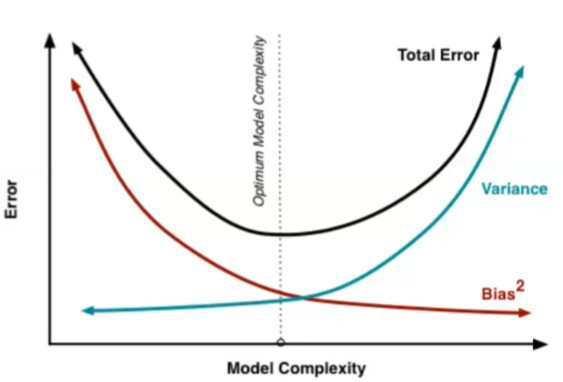
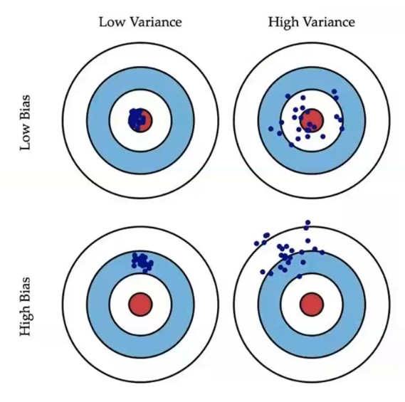
Error, variance and deviation

loss = bias + variance

Expected value of error = variance of noise + variance of model predicted value + square of deviation of predicted value from real value

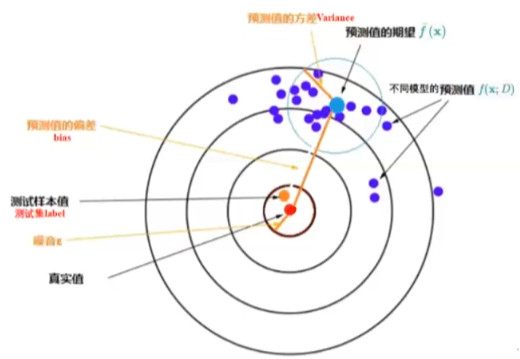
• Red dot: true value of test sample
• Orange dot: true value of test sample + noise
• Purple point: each specific model predicts the test sample once, which corresponds to a point
• Blue dot: average of all predicted values [expectation of predicted values]
• Light blue circle: the dispersion of the predicted value, that is, the variance of the predicted value

Deviation:

The deviation reflects the error between the output of the model and the real value.

How to reduce?

• Increase the complexity of the algorithm
  For example, linear regression increases the number of parameters to improve the complexity of the model; Neural network increases the complexity of the model by increasing the number of hidden units.
• Optimize input features - > add more features
• Weakening or removing existing regularization constraints = > may increase variance
• Adjust model structure

Variance:

The larger the variance, the easier it is to over fit the model.

In case of large variance and over fitting:

• Increasing the amount of data in the training set will not affect the deviation.
• Regularization, the model is too biased towards the regular term, which may affect the deviation
• A variety of model training data are used, and the final model is selected by means of cross validation

Regularization:

In order to reduce the complexity of the model.

Challenges of machine learning

• Training error refers to the error on the training set = > under fitting, and the model cannot obtain sufficient error on the training set
• Test error refers to the error on the test set = > over fitting, and the gap between training error and test error is too large

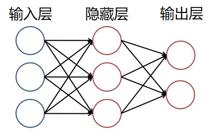
Fundamentals of neural network

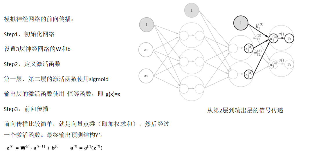
Using numpy to simulate forward propagation

Activation function

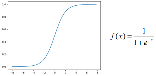
sigmoid

characteristic:

• The input is a continuous real value, and the output result is between 0 and 1
• The output result of negative infinity is 0, and the output result of positive infinity is 1

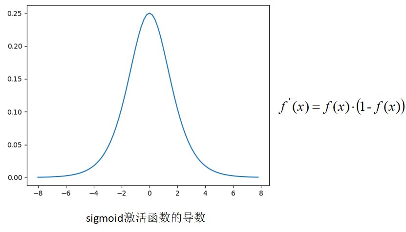
• If the weight of the initial neural network is a random value between [0,1], it can be seen from the back-propagation algorithm that when the gradient propagates from back to front, the gradient value of each layer will be reduced to 0.25 times of the original. If the neural network has many layers, the gradient will become very small (close to 0) after multi-layer propagation, that is, the gradient disappears

• When the network weight is initialized to the value in the (1, + ∞) interval, a gradient explosion will occur

tanh:

• y=tanh(x) is an odd function, that is, the strictly monotonic increasing curve of the image passing through the origin and passing through the first and third quadrants
• Also known as hyperbolic tangent function, the function curve is similar to Sigmoid function and can be transformed by scaling and translation

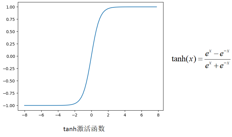
• Compared with sigmoid function, the mean of tanh is 0
• tanh is easier to train than Sigmoid function and has advantages
• It is used for normalized regression problem, and its output is in the range of [- 1,1]. Usually used with L2 loss

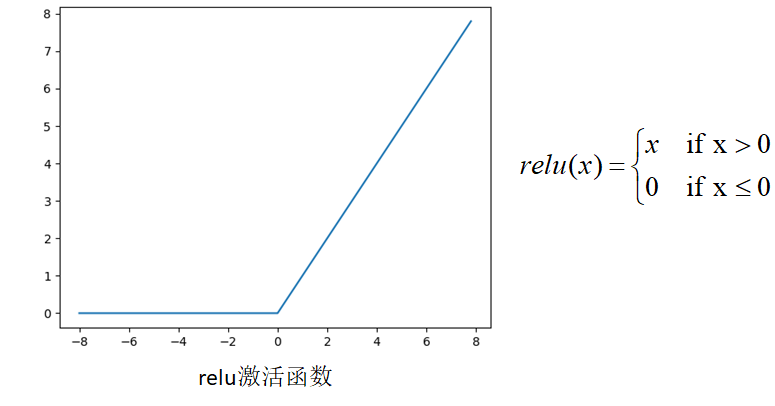
relu:

• Unilateral suppression, the sparse model realized by ReLU can better mine relevant features and fit training data

• For linear functions, ReLU has stronger expression ability, especially in depth networks

• For the nonlinear function, because the gradient of the non negative interval of ReLU is constant, there is no gradient disappearance problem, so that the convergence rate of the model is maintained in a stable state

To sum up:

• The output values of sigmoid and tanh functions are between (0,1) and (- 1,1) = > suitable for processing probability values; Gradient vanishing = > not suitable for deep network training
• The effective derivative of relu is constant 1, which solves the gradient disappearance problem in deep network = > it is more suitable for deep network training

Gradient disappearance

• When the gradient is less than 1, the error between the predicted value and the real value will decay once per propagation layer. This phenomenon is particularly obvious if sigmoid is used as the activation function in the deep model, which will lead to the stagnation of model convergence
• When the gradient disappears, the weight update of the hidden layer close to the output layer is relatively normal because its gradient is relatively normal. However, when it is closer to the input layer, the weight update of the hidden layer close to the input layer will be slow or stagnant due to the disappearance of the gradient = > this will only be equivalent to the learning of the shallow network of the following layers during training

Why do we need to use nonlinear activation functions in neural networks?

• If the activation function is not used, it is equivalent to the excitation function f(x) = x. at this time, the input of each layer node is the linear function of the output of the upper layer. Then, no matter how many layers the neural network has, the output is the linear combination of inputs = > which is equivalent to the effect of no hidden layer
• The nonlinear function is introduced as the excitation function, so the expression ability of neural network will be more powerful = > it is no longer a linear combination of inputs, but can approximate almost any function

Complete neural network learning process

1. Define the network structure (specify the size of output layer, hidden layer and output layer)

2. Initialize model parameters

3. Cyclic operation:

   3.1 implementation of forward communication

   3.2 calculation of loss function

   3.3 post implementation communication

   3.4 weight update

Back propagation

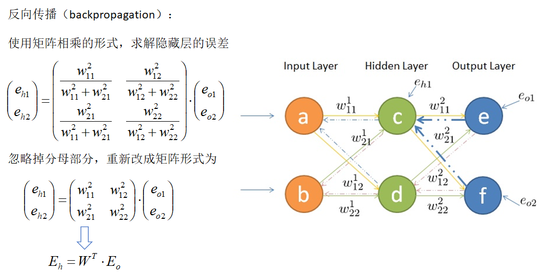
Function of weight matrix

• Forward propagation: transmitting input signals
• Back propagation: error in transmitting output

Using numpy to implement a neural network

import numpy as np
import matplotlib.pyplot as plt

if __name__ == '__main__':
    #n: Sample size; d_in: enter a dimension; h: Hidden layer dimension; d_out: output dimension
    n,d_in,h,d_out = 64,1000,100,10
    #Randomly generated data
    x = np.random.randn(n,d_in)  # n line d_in column with standard normal distribution
    y = np.random.randn(n,d_out) # n line d_out column with standard normal distribution
    #print(x)
    #Random initialization weight
    w1  = np.random.randn(d_in,h) #Enter layer to hidden layer weights
    w2  = np.random.randn(h,d_out) #Hide layer to output layer weights
    #Set learning rate
    learn_rate = 1e-6
    #Number of iterations
    times = 200
    for i in range(times):
        #Forward propagation calculation predicted value y
        temp = x.dot(w1)
        temp_relu = np.maximum(temp,0) #Compare the size of two array s element by element. If it is less than 0, it is 0
        y_pred = temp_relu.dot(w2)
        #Calculation loss function
        loss = np.square(y_pred - y).sum() / n
        print(i,loss)
        #Back propagation
        grad_y_pred = 2.0 * (y_pred - y)
        #Calculate w2 gradient
        grad_w2 = temp_relu.T.dot(grad_y_pred)
        grad_temp_relu = grad_y_pred.dot(w2.T)
        grad_temp = grad_temp_relu.copy()
        #relu activation function, less than 0 is 0
        grad_temp[temp < 0] = 0
        #Calculate w1 gradient
        grad_w1 = x.T.dot(grad_temp)
        #Update weight
        w1 -= learn_rate * grad_w1
        w2 -= learn_rate * grad_w2
    print(w1,w2)

Using numpy to complete boston house price prediction based on Neural Network

import numpy as np
import matplotlib.pyplot as plt
from sklearn.datasets import load_boston
from sklearn.utils import shuffle, resample

# relu function
def Relu(x):
    res = np.where(x < 0,0,x)
    return res
# Define loss function
def MSE_loss(y, y_hat):
    return np.mean(np.square(y_hat - y))
# Define linear regression function
def Linear(X, W1, b1):
    y = X.dot(W1) + b1
    return y

if __name__ == '__main__':
    #Data loading
    data = load_boston()
    X_ = data['data']
    y = data['target']
    #Convert y to matrix form
    y = y.reshape(y.shape[0],1) #shape[0] read the length of dimension 0 reshape: modify to the specified dimension size
    #Data normalization axis = 0: compress rows, calculate the mean value of each column, and return a matrix of 1*n
    X_ = (X_ - np.mean(X_,axis=0)) / np.std(X_,axis=0)
    """
        Initialize network parameters
        Define hidden layer dimensions n_hidden，w1,b1,w2,b2
    """
    n_features = X_.shape[1] #Gets the dimension size of the column, that is, the number of features
    n_hidden = 10
    w1 = np.random.randn(n_features, n_hidden)
    b1 = np.zeros(n_hidden)
    w2 = np.random.randn(n_hidden, 1)
    b2 = np.zeros(1)
    # Set learning rate
    learning_rate = 1e-6
    # 5000 iterations
    for t in range(5000):
        # Forward propagation, calculate the predicted value Y (linear - > relu - > linear)
        l1 = Linear(X_,w1,b1)
        s1 = Relu(l1)
        y_pred = Linear(s1,w2,b2)
        # Calculate the loss function and output the loss of each epoch
        loss = MSE_loss(y,y_pred)
        # Back propagation, calculate the gradient of w1 and w2 based on loss
        grad_y_pred = 2 *(y_pred - y)
        grad_w2 = s1.T.dot(grad_y_pred)
        grad_temp_relu = grad_y_pred.dot(w2.T)
        grad_temp_relu[l1 < 0] = 0
        grad_w1 = X_.T.dot(grad_temp_relu)
        # Update the weight and update W1, W2, B1 and B2
        w1 = w1 - learning_rate * grad_w1
        w2 = w2 - learning_rate * grad_w2
    # Get the final w1, w2
    print('w1={} \n w2={}'.format(w1, w2))

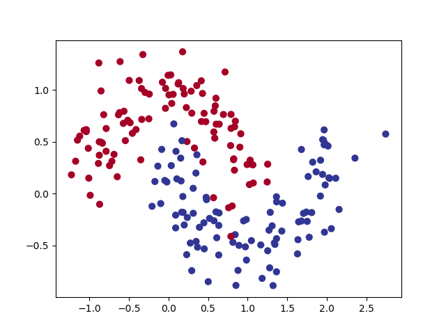
Binary classification using PyTorch custom neural network

from sklearn.datasets import make_moons
import torch
import numpy as np
import matplotlib.pyplot as plt
import torch.nn as nn
import torch.nn.functional as F
from sklearn.metrics import accuracy_score

#Define the network model and inherit nn.Module
class Net(nn.Module):
    #initialization
    def __init__(self):
        super(Net,self).__init__()
        #Define the first FC layer and use Linear transformation
        self.fc1 = nn.Linear(2,100)
        #Define the second FC layer and use Linear transformation
        self.fc2 = nn.Linear(100,2)
    #Forward propagation
    def forward(self,x):
        #Layer 1 output
        x = self.fc1(x)
        #Active layer
        x = torch.tanh(x)
        #Output layer
        x = self.fc2(x)
        return x
    #Prediction results
    def predict(self,x):
        pred = self.forward(x)
        ans = []
        for t in pred:
            if t[0] > t[1]:
                ans.append(0)
            else:
                ans.append(1)
        return torch.tensor(ans)

# Predict and convert to numpy type
def predict(x):
    x = torch.from_numpy(x).type(torch.FloatTensor)
    ans = model.predict(x)
    return ans.numpy()

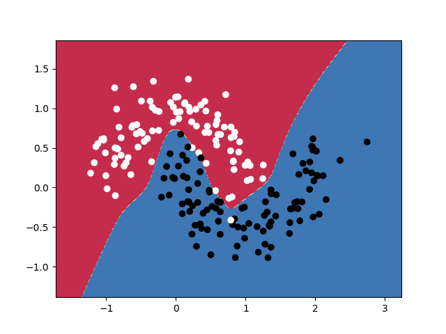
# Draw two classification decision surface
def plot_decision_boundary(pred_func, X, y):
    # Set min and max values and give it some padding
    x_min, x_max = X[:, 0].min() - .5, X[:, 0].max() + .5
    y_min, y_max = X[:, 1].min() - .5, X[:, 1].max() + .5
    h = 0.01
    # Calculation decision surface
    xx, yy = np.meshgrid(np.arange(x_min, x_max, h), np.arange(y_min, y_max, h))
    # np.c_ Connecting two matrices by row is to add the two matrices left and right
    Z = pred_func(np.c_[xx.ravel(), yy.ravel()])
    Z = Z.reshape(xx.shape)
    # Draw classification decision surface
    plt.contourf(xx, yy, Z, cmap=plt.cm.Spectral)
    # Draw sample points
    plt.scatter(X[:, 0], X[:, 1], c=y, cmap=plt.cm.binary)
    plt.show()


if __name__ == '__main__':
    # Using make_moon built-in generation model randomly generates binary data and 200 samples
    np.random.seed(33)
    X,y = make_moons(200,noise=0.2)
    print(y)
    cm = plt.cm.get_cmap('RdYlBu')
    #X[:,0]: take the 0th data from all arrays X[:,1]: take the 1st data from all arrays
    plt.scatter(X[:,0],X[:,1],s=40,c=y,cmap=cm)
    plt.show()
    #Arrays are converted to tensors, and they share memory
    X = torch.from_numpy(X).type(torch.FloatTensor)
    y = torch.from_numpy(y).type(torch.LongTensor)
    #Initialization model
    model = Net()
    #Define evaluation criteria
    criterion = nn.CrossEntropyLoss()
    #Define optimizer
    print(f'\nParameters: {np.sum([param.numel() for param in model.parameters()])}')
    optimizer = torch.optim.Adam(model.parameters(), lr=0.01)
    #Number of iterations
    times = 1000
    #Store loss per iteration
    losses = []
    for i in range(times):
        #Predict the input x
        y_pred = model.forward(X)
        #The loss function is obtained
        loss = criterion(y_pred,y)
        losses.append(loss.item())
        #Gradient before emptying
        optimizer.zero_grad()
        #Calculated gradient
        loss.backward()
        #Adjust weight
        optimizer.step()
    print(model.predict(X))
    print(accuracy_score(model.predict(X), y))
    plot_decision_boundary(lambda x: predict(x), X.numpy(), y.numpy())

Output results: