Modern neural network

This week, I mainly learned several classic modern neural networks: AlexNet, VGG, NiN, geoglenet and ResNet.
These networks can be regarded as a process of continuous refinement in the development of neural networks:
Starting from the LeNet network, AlexNet is generated by changing the activation function and using DropOut and other methods;
After introducing the concept of block, VGG block is constructed to realize the regular VGGNet of the network;
In order to reduce the parameters, two 1 * 1 convolution layers are used to replace the NiN of the full connection layer;
And then to the implementation of GoogleNet combined with the concept of multiple paths;
Then to ResNet, which takes the input parameters into account;
This change is to make the network deeper and more optimized, so as to obtain better implementation performance.
Learn AI from Li Mu - hands on deep learning - modern neural network

Using ResNet for transfer learning to realize cat dog war classification

The first is to learn the code of cat dog war classification given by the teacher using VGG for migration learning.
Sort out the code ideas through learning, and then further modify the model.

VGG's idea of transfer learning:

Data download: https://god.yanxishe.com/8
Data preprocessing: use transforms to cut the size of 224 * 224 and convert CHW format.
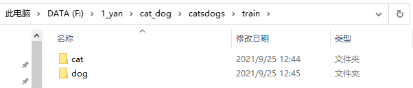
Data local operation: the training data is 900 pictures of cats and 900 pictures of dogs, and the data is set to the architecture of train/dog and train/cat.
Transfer learning: operate with vgg16, fix the convolution at the front, train the Linear at the back, and finally operate softmax.

ResNet migration learning implementation:

The overall idea is similar to that of using vgg for transfer learning.
The code implementation mainly refers to VGG's migration learning and blog: https://www.cnblogs.com/Arsene-W/p/13377011.html

1. Import the required package

#1. Import package, set gpu/cpu, set random seed
import numpy as np
import matplotlib.pyplot as plt
import os
import torch
import torch.nn as nn
import torchvision
from torchvision import models,transforms,datasets
import time
import json
import shutil
from PIL import Image
import csv

# Determine whether there is a GPU device
device = torch.device("cuda:0" if torch.cuda.is_available() else "cpu")
print('Using gpu: %s ' % torch.cuda.is_available())
# Set random seeds for easy reproduction
torch.manual_seed(10000)            # Set random seed for CPU
torch.cuda.manual_seed(10000)       # Set random seed for current GPU
torch.cuda.manual_seed_all(10000)   # Set random seed for all GPU s

1. Data download. The data is already local, but compared with the vgg migration learning code run by collab with cpu, the training data used here is changed to 500 cats and 500 dogs, because the local gpu can't stand it.
   
2. Load the dataset and process the data

#3. Load the data set and process the data
normalize = transforms.Normalize(mean=[0.485, 0.456, 0.406], std=[0.229, 0.224, 0.225])
#Function: standardize the image channel by channel (the mean becomes 0 and the standard deviation becomes 1), which can speed up the convergence of the model.
#Mean: mean value of each channel, std: standard deviation of each channel, inplace: whether to operate in situ.
#Think about the question: Why are the values in mean and std like this? This set of data is sampled from the ImageNet training set.
resnet_format = transforms.Compose([
                transforms.CenterCrop(224),
                transforms.ToTensor(),
                normalize,
            ])
#The torchvision.transforms.Compose () class is mainly used to concatenate multiple picture transformations.
#The construction of this class is very simple:
#transforms.CenterCrop is mainly used to cut the image from the center to 224 * 224
#transforms.ToTensor is mainly: first convert from HWC to CHW format, then to float type, and finally divide each pixel by 255.

data_dir = r'F:\1_yan\cat_dog\catsdogs'

dsets = {x: datasets.ImageFolder(os.path.join(data_dir, x), resnet_format)
         for x in ['train', 'val']}
#datasets.ImageFolder(root,transform,target_transform,loader,is_valid_file)
#Root: the root directory of image storage, that is, the directory above the directory where each category folder is located.
#transform: an operation (function) that preprocesses an image. The original image is used as input to return a converted image.
#target_transform: the operation of preprocessing the picture category. The input is target and the output is the conversion. If this parameter is not passed, i.e. no conversion is made to the target, the returned order index is 0, 1, 2
#loader: indicates the loading method of the dataset. Generally, the default loading method is OK.
#is_valid_file: a function that gets the path of the image file and checks whether the file is a valid file (that is, it is used to check for damaged files).
dset_sizes = {x: len(dsets[x]) for x in ['train', 'val']}
dset_classes = dsets['train'].classes

#Under resnet50, the display memory needs to be too large. Reduce the batch size to 5
loader_train = torch.utils.data.DataLoader(dsets['train'], batch_size=5, shuffle=True, num_workers=4)
loader_valid = torch.utils.data.DataLoader(dsets['val'], batch_size=5, shuffle=False, num_workers=4)

1. Load ResNet50 and modify the full connection layer of the model

#4. Load ResNet152 and modify the full connection layer of the model
#model = models.resnet152(pretrained=True)
model = models.resnet50(pretrained=True)
model_new = model.to(device);
model_new.fc = nn.Linear(2048, 2,bias=True)
model_new = model_new.to(device)
print(model_new)

#Partial parameters
#Cross entropy loss function
criterion = nn.CrossEntropyLoss()
#The loss function combines nn.LogSoftmax() and nn.NLLLoss(). It is very useful when doing classification (specific categories) training.
# Learning rate: 0.001, every 10epoch *0.1
lr = 0.001

# Random gradient descent, momentum accelerated learning, Weight decay to prevent over fitting
optimizer = torch.optim.SGD(model_new.parameters(), lr=lr, momentum=0.9, weight_decay=5e-4)

1. model training

#5. Model training
def val_model(model,dataloader,size):
    model.eval()
    predictions = np.zeros(size)
    all_classes = np.zeros(size)
    all_proba = np.zeros((size,2))
    i = 0
    running_loss = 0.0
    running_corrects = 0
    with torch.no_grad():
        for inputs,classes in dataloader:
            inputs = inputs.to(device)
            classes = classes.to(device)
            outputs = model(inputs)
            loss = criterion(outputs,classes)           
            _,preds = torch.max(outputs.data,1)
            # statistics
            running_loss += loss.data.item()
            running_corrects += torch.sum(preds == classes.data)
            #predictions[i:i+len(classes)] = preds.to('cpu').numpy()
            #all_classes[i:i+len(classes)] = classes.to('cpu').numpy()
            #all_proba[i:i+len(classes),:] = outputs.data.to('cpu').numpy()
            i += len(classes)
            #print('Testing: No. ', i, ' process ... total: ', size)        
    epoch_loss = running_loss / size
    epoch_acc = running_corrects.data.item() / size
    #print('Loss: {:.4f} Acc: {:.4f}'.format(epoch_loss, epoch_acc))
    return epoch_loss, epoch_acc 


def train_model(model,dataloader,size,epochs=1,optimizer=None):
    
    
    for epoch in range(epochs):
        model.train()
        
        running_loss = 0.0
        running_corrects = 0
        count = 0
        for inputs,classes in dataloader:
            inputs = inputs.to(device)
            classes = classes.to(device)
            outputs = model(inputs)
            loss = criterion(outputs,classes)           
            optimizer = optimizer
            optimizer.zero_grad()
            loss.backward()
            optimizer.step()
            _,preds = torch.max(outputs.data,1)
            # statistics
            running_loss += loss.data.item()
            running_corrects += torch.sum(preds == classes.data)
            count += len(inputs)
            print('Training: No. ', count, ' process ... total: ', size)
        epoch_loss = running_loss / size
        epoch_acc = running_corrects.data.item() / size
        epoch_Valloss, epoch_Valacc = val_model(model,loader_valid,dset_sizes['val'])
        print('epoch: ',epoch,' Loss: {:.5f} Acc: {:.5f} ValLoss: {:.5f} ValAcc: {:.5f}'.format(
                     epoch_loss, epoch_acc,epoch_Valloss,epoch_Valacc))
        scheduler.step()
 
#Learning rate attenuation
scheduler = torch.optim.lr_scheduler.StepLR(optimizer, step_size=10, gamma=0.1) 

# model training
train_model(model_new,loader_train,size=dset_sizes['train'], epochs=1 , 
            optimizer=optimizer)       

1. Model test and output csv file

#6. Test the model and output the csv file
model_new.eval()
csvfile = open('csv.csv', 'w') 
writer = csv.writer(csvfile)
test_root='F:/1_yan/cat_dog/cat_dog/test/'
img_test=os.listdir(test_root)
img_test.sort(key= lambda x:int(x[:-4]))
for i in range(len(img_test)):
    img = Image.open(test_root+img_test[i]) 
    img = img.convert('RGB')
    input=resnet_format(img)
    input=input.unsqueeze(0)
    input = input.to(device)
    output=model_new(input)
    _,pred = torch.max(output.data,1)
    print(i,pred.tolist()[0])
    writer.writerow([i,pred.tolist()[0]])
csvfile.close()

1. Submit results
   

summary

1. This week I learned and understood several modern neural network structures, but I still don't understand their implementation and use.
2. Learning and understanding of transfer learning, using ResNet for transfer learning to achieve cat dog war, but it's not clear why the effect is good...
3. There are still deficiencies in the use of pytoch. Now we often look at the source code and don't know where to search.