Data visualization is an important part of the work of data scientists. In the early stages of a project, you usually do Exploratory Data Analysis (EDA) to get some understanding of the data. Creating visualization methods really helps to make things clearer and easier to understand, especially for large, high-dimensional datasets. At the end of the project, it is important to present the final results in a clear, concise and compelling way, because your audience is often non-technical customers, so that they can understand.
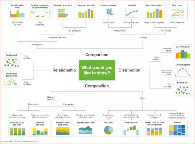
Matplotlib is a popular Python library that can be used to easily create data visualization solutions. But every time a new project is created, setting up data, parameters, graphics and typesetting becomes cumbersome and cumbersome. In this blog post, we will focus on five data visualization methods and use Python Matplotlib to write some quick and simple functions for them. At the same time, here's a great chart for choosing the right visualization method in your work!
Enter the group: 5148377875, you can get dozens of PDF s!
The scatter plot is very suitable for showing the relationship between the two variables, because you can see the original distribution of the data directly. As shown in the first figure below, you can also see the relationship between different groups of data by simply color coding the groups. Want to visualize the relationships among the three variables? No problem! The third variable can be coded using only another parameter, such as point size, as shown in the second figure below.
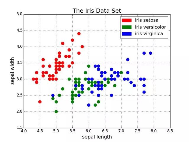
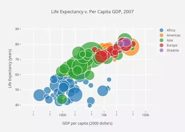
Now let's start talking about the code. We first import Matplotlib's pyplot with the alias "plt". To create a new bitmap, we can call plt.subplots(). We pass the x- and y-axis data to the function, and then pass the data to ax.scatter() to plot the scatter plot. We can also set the size, color and alpha transparency of the dots. You can even set the Y axis to a logarithmic scale. Titles and labels on coordinate axes can be set specifically for this figure. This is an easy-to-use function that can be used to create scatter plots from beginning to end!
import matplotlib.pyplot as pltimport numpy as npdef scatterplot(x_data, y_data, x_label="", y_label="",title="", color = "r", yscale_log=False):
# Create the plot object
_, ax = plt.subplots() # Plot the data, set the size (s), color and transparency (alpha)
# of the points
ax.scatter(x_data, y_data, s = 10, color = color, alpha = 0.75) if yscale_log == True:
ax.set_yscale('log') # Label the axes and provide a title
ax.set_title(title)
ax.set_xlabel(x_label)
ax.set_ylabel(y_label)
Broken line diagram
When you can see that one variable changes significantly with another variable, for example, they have a large covariance, it's better to use a polygraph. Let's take a look at the picture below. We can clearly see that for all the main lines there are a lot of changes over time. Using scatters to draw these will be extremely confusing and difficult to really understand and see what's happening. Breakdown charts are very good for this situation, because they basically provide us with a quick summary of the covariance of the two variables (percentage and time). In addition, we can also group by color coding.

Here is the code for the line chart. It is very similar to the scatter plot above, except that there are minor variations in some variables.
def lineplot(x_data, y_data, x_label="", y_label="", title=""):
# Create the plot object
_, ax = plt.subplots() # Plot the best fit line, set the linewidth (lw), color and
# transparency (alpha) of the line
ax.plot(x_data, y_data, lw = 2, color = '#539caf', alpha = 1) # Label the axes and provide a title
ax.set_title(title)
ax.set_xlabel(x_label)
ax.set_ylabel(y_label)
histogram
Histograms are useful for viewing (or really exploring) the distribution of data points. Look at the histogram we made with frequency and IQ below. We can clearly see the aggregation toward the middle, and we can see what the median is. We can also see that it has a normal distribution. The histogram can clearly show the relative differences of frequencies among groups. The use of groups (discretization) really helps us see "more macroscopic graphics", but when we use all data points without discrete groups, it may cause a lot of interference to visualization, making it difficult to see what is happening in the hall.
The following is the histogram code in Matplotlib. There are two parameters to note: first, the parameter n_bins controls how many discrete groups we want in the histogram. More groups will provide us with better information, but may also introduce interference to keep us away from the overall situation; on the other hand, fewer groups will give us a more "bird's-eye view" and a global picture without more details. Secondly, the parameter cumulative is a Boolean value, which allows us to choose whether the histogram is cumulative or not. Basically, the choice is PDF (Probability Density Function) or CDF (Cumulative Density Function).
def histogram(data, n_bins, cumulative=False, x_label = "", y_label = "", title = ""):
_, ax = plt.subplots()
ax.hist(data, n_bins = n_bins, cumulative = cumulative, color = '#539caf')
ax.set_ylabel(y_label)
ax.set_xlabel(x_label)
ax.set_title(title)
Imagine that we want to compare the distribution of two variables in the data. One might think that you have to make two histograms and compare them side by side. However, there is actually a better way: we can overlay histograms with different transparencies. Look at the figure below. The transparency of the uniform distribution is set to 0.5, so that we can see the figure behind him. So we can see two distributions directly in the same chart.
For overlapping histograms, something needs to be set up. First, we set the horizontal axis range that can accommodate different distributions at the same time. Based on this range and the expected number of groups, we can really calculate the width of each group. Finally, we draw two histograms on the same graph, one of which is slightly more transparent.
# Overlay 2 histograms to compare themdef overlaid_histogram(data1, data2, n_bins = 0, data1_name="", data1_color="#539caf", data2_name="", data2_color="#7663b0", x_label="", y_label="", title=""):
# Set the bounds for the bins so that the two distributions are fairly compared
max_nbins = 10
data_range = [min(min(data1), min(data2)), max(max(data1), max(data2))]
binwidth = (data_range[1] - data_range[0]) / max_nbins if n_bins == 0
bins = np.arange(data_range[0], data_range[1] + binwidth, binwidth) else:
bins = n_bins # Create the plot
_, ax = plt.subplots()
ax.hist(data1, bins = bins, color = data1_color, alpha = 1, label = data1_name)
ax.hist(data2, bins = bins, color = data2_color, alpha = 0.75, label = data2_name)
ax.set_ylabel(y_label)
ax.set_xlabel(x_label)
ax.set_title(title)
ax.legend(loc = 'best')
Histogram
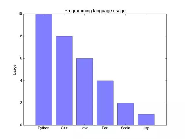
Histograms are most effective when you try to visualize classification data with very few categories (possibly less than 10). If we have too many classifications, these histograms will be very cluttered and difficult to understand. Column graphs are good for classification data because you can easily see the differences between column-based categories (such as size); classification is also easy to divide and encode with color. We'll see three different types of histograms: regular, grouped, stacked. As we proceed, please look at the code below the graph.
The conventional bar chart is shown in Figure 1 below. In the barplot() function, xdata represents the mark on the x axis, and ydata represents the height of the rod on the y axis. The error bar is an additional line centered on each column, which can draw the standard deviation.
Grouped histograms allow us to compare multiple classification variables. Look at Figure 2 below. The first variable we compared was how the scores of different groups changed (groups G1, G2,...). And so on. We're also comparing gender and color codes. Looking at the code, the y_data_list variable is actually a list of Y elements, each of which represents a different group. Then we loop through each group, and for each group, we draw each tag on the x-axis; each group is coded in color.
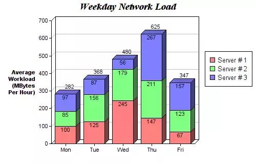
Stacked histograms can be used to observe the classification of different variables. In the stacked bar chart in Figure 3, we compared the server load on a daily basis. Through the color-coded stack diagram, we can easily see and understand which servers work the most every day, and compare the load with other servers. The code for this code is the same as the bar graph for the grouping. We cycle through each group, but this time we put the new columns on the old ones instead of next to them.
def barplot(x_data, y_data, error_data, x_label="", y_label="", title=""):
_, ax = plt.subplots()
# Draw bars, position them in the center of the tick mark on the x-axis
ax.bar(x_data, y_data, color = '#539caf', align = 'center')
# Draw error bars to show standard deviation, set ls to 'none'
# to remove line between points
ax.errorbar(x_data, y_data, yerr = error_data, color = '#297083', ls = 'none', lw = 2, capthick = 2)
ax.set_ylabel(y_label)
ax.set_xlabel(x_label)
ax.set_title(title)
def stackedbarplot(x_data, y_data_list, colors, y_data_names="", x_label="", y_label="", title=""):
_, ax = plt.subplots()
# Draw bars, one category at a time
for i in range(0, len(y_data_list)):
if i == 0:
ax.bar(x_data, y_data_list[i], color = colors[i], align = 'center', label = y_data_names[i])
else:
# For each category after the first, the bottom of the
# bar will be the top of the last category
ax.bar(x_data, y_data_list[i], color = colors[i], bottom = y_data_list[i - 1], align = 'center', label =y_data_names[i])
ax.set_ylabel(y_label)
ax.set_xlabel(x_label)
ax.set_title(title)
ax.legend(loc = 'upper right')
def groupedbarplot(x_data, y_data_list, colors, y_data_names="", x_label="", y_label="", title=""):
_, ax = plt.subplots()
# Total width for all bars at one x location
total_width = 0.8
# Width of each individual bar
ind_width = total_width / len(y_data_list)
# This centers each cluster of bars about the x tick mark
alteration = np.arange(-(total_width/2), total_width/2, ind_width)
# Draw bars, one category at a time
for i in range(0, len(y_data_list)):
# Move the bar to the right on the x-axis so it doesn't
# overlap with previously drawn ones
ax.bar(x_data + alteration[i], y_data_list[i], color = colors[i], label = y_data_names[i], width =ind_width)
ax.set_ylabel(y_label)
ax.set_xlabel(x_label)
ax.set_title(title)
ax.legend(loc = 'upper right')
Box diagram
We looked at the histogram before, which visualizes the distribution of variables very well. But what if we need more information? Maybe we want to see the standard deviation more clearly? Maybe the median is very different from the mean. Do we have many outliers? What if such an offset and many values are concentrated on one side?
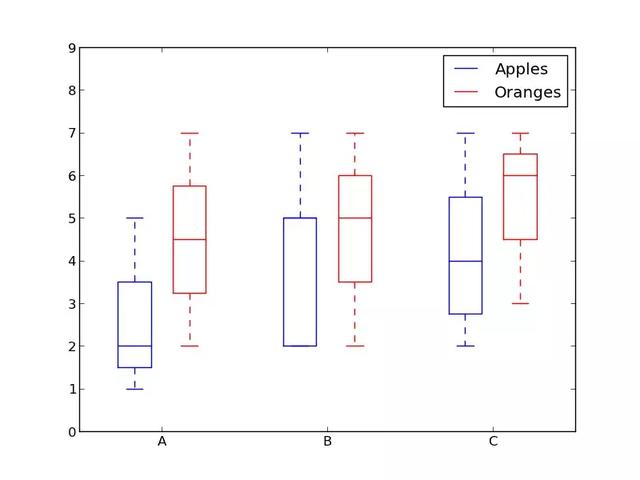
That's what boxes are good for. The box diagram gives us all the information above. The bottom and top of a solid wire frame are always the first and third quartile (such as 25% and 75% data), and the horizontal line in the box is always the second quartile (median). Lines like whiskers (dotted lines and end lines) protrude from the box to show the range of data.
Because the block diagrams of each group/variable are drawn separately, it is easy to set them up. xdata is a list of groups / variables. The box plot () function of the Matplotlib library draws a box for each column or vector in ydata. Therefore, each value in xdata corresponds to a column / vector in ydata. What we need to set up is the beauty of the box.
def boxplot(x_data, y_data, base_color="#539caf", median_color="#297083", x_label="", y_label="",title=""):
_, ax = plt.subplots()
# Draw boxplots, specifying desired style
ax.boxplot(y_data
# patch_artist must be True to control box fill
, patch_artist = True
# Properties of median line
, medianprops = {'color': median_color}
# Properties of box
, boxprops = {'color': base_color, 'facecolor': base_color}
# Properties of whiskers
, whiskerprops = {'color': base_color}
# Properties of whisker caps
, capprops = {'color': base_color})
# By default, the tick label starts at 1 and increments by 1 for
# each box drawn. This sets the labels to the ones we want
ax.set_xticklabels(x_data)
ax.set_ylabel(y_label)
ax.set_xlabel(x_label)
ax.set_title(title)
epilogue
There are five fast and simple data visualization methods using Matplotlib. Abstracting related transactions into functions always makes your code easier to read and use! I hope you enjoyed this article and learned some useful new skills. If you do, please feel free to give it a compliment.