Feature Selection of Python Sklearner Learning

1. Removing low variance features

Variance Threshold is a simple and basic method for feature selection, which removes all features whose variances do not meet some thresholds. By default, it removes all zero-variance features (the same value), i.e. those that are invariant on all samples.

from sklearn.feature_selection import VarianceThreshold

X = [[0, 2, 0, 3], [0, 1, 4, 3], [0, 1, 1, 3], [0, 2, 3, 3]]
select = VarianceThreshold()
result = select.fit_transform(X)
print(result)

[[2 0]
 [1 4]
 [1 1]
 [2 3]]

Variance Threshold plays the following roles in the above code:

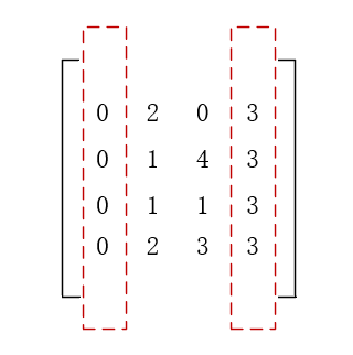
The first and fourth column features are removed and the middle two columns are selected.

• VarianceThreshold class definition

def __init__(self, threshold=0.):

• Description of parameters

VarianceThreshold object can be created with a parameter threshold. This parameter defines a threshold, which defaults to 0. If it is set manually, the feature whose variance in training set is lower than the threshold will be deleted.

• Example

Assuming that we have a data set with Boolean values, we want to remove features that have a ratio of 0 or 1 in the whole data set that is more than 80%. The Boolean characteristic is Bernoulli random variable. The variance of the variable is Var[X]=p(1_p) Var[X]=p(1-p) Var[X]=p(1_p).
So, the whole code is as follows: (the probability of the median value of the first column being 0 is p = 5/6 > 8)

from sklearn.feature_selection import VarianceThreshold

X = [[0, 0, 1], [0, 1, 0], [1, 0, 0], [0, 1, 1], [0, 1, 0], [0, 1, 1]]
select = VarianceThreshold(.8 * (1 - .8))
result = select.fit_transform(X)
print(result)

[[0 1]
 [1 0]
 [0 0]
 [1 1]
 [1 0]
 [1 1]]

2. Univariate feature selection

2.1 Univariate Feature Selection Tool Class

Univariate feature selection is essentially a test for each variable (feature), such as chi-square test, to get a test result (score). Choose the features we need based on this score.
Common tool classes are as follows:

• SelectKBest(self, score_func=f_classif, k=10): Use the test function specified by score_func to detect each feature, retaining the K with the highest score (default is 10)
• SelectPercentile(self, score_func=f_classif, percentile=10): Each feature is detected with the test function specified by score_func, retaining the features of the first few percent, with the percentage specified by percentile (default is% 10).
• SelectFpr(self, score_func=f_classif, alpha=5e-2): According to the FPR test, select the pvalues lower than alpha, where the FPR test represents the false positive rate test, which controls the total amount of error detection.
• SelectFdr(score_func=f_classif, alpha=0.05): Select the p value of the estimated error detection rate, where alpha represents the highest uncorrected p value of the function to be retained.
• SelectFwe(score_func=f_classif, alpha=0.05): Select the p value corresponding to the family error rate, where alpha represents the p value of the feature score.
• Generic Univariate Select (score_func=f_classif, mode='percentile', param=1e-05): This is a configurable single variable feature selector, which is checked with the specified score_func test function, and then retains the required features according to the mode specified way, in which mode takes the values {percentile', `k_best', `fpr, 'fdr','fwe'} and param are parameters corresponding to different modes

2.2 score_func parameter description

2.2.1 for regression:

• f_regression: Univariate Linear Regression

I=((X[:,i]−mean(X[:,i]))∗(y−meany))/(std(X[:,i])∗std(y)) I = ((X[:, i] - mean(X[:, i])) * (y - mean_y)) / (std(X[:, i]) * std(y)) I=((X[:,i]−mean(X[:,i]))∗(y−meany​))/(std(X[:,i])∗std(y))

• mutual_info_regression: Estimate the mutual information of continuous target variables. Mutual information describes the dependence between two variables. If and only if two random variables are independent, the mutual information value is 0. The greater the value, the greater the dependence.

I(X;Y)=∫Y∫Xp(x,y)log(p(x,y)p(x),p(y))dxdy I(X;Y) = \int_{Y} \int_{X}p(x,y)log({{p(x,y)}\over{p(x),p(y)}})dxdy I(X;Y)=∫Y​∫X​p(x,y)log(p(x),p(y)p(x,y)​)dxdy

Among them, p(x,y) is the joint probability density function of X and Y, while p(x) and p(y) are the edge probability density functions of X and Y, respectively.

2.2.2 For classification:

• Chi 2: Calculate the chi-square statistics between each non-negative feature.

X2=∑i=1k(fi−npi2)npi X^2 = \sum^k_{i=1}{({f_i-np_i}^2) \over np_i} X2=i=1∑k​npi​(fi​−npi​2)​

It is assumed that the overall distribution is F(x)F(x)F(x) F(x), and that the overall distribution rate of X is P{X=x i}=pi, i=1,2,3,... P{X=x_i}=p_i, i=1,2,3,... P{X=xi}=pi, i=1,2,3,....

• f_classif: Calculate the ANOVA F value of the sample provided (ANOVA), which is the default function of the above test tool class. It calculates the ratio of the mean variance between groups to the mean variance within groups.
• mutual_info_classif: Estimating Mutual Information of Discrete Target Variables

I(X;Y)=∑y∈Y∑x∈Xlog(p(x,y)p(x),p(y)) I(X;Y) = \sum_{y \in Y} \sum_{x \in X}log({{p(x,y)}\over{p(x),p(y)}}) I(X;Y)=y∈Y∑​x∈X∑​log(p(x),p(y)p(x,y)​)

Among them, p(x,y) is the joint probability distribution function of X and Y, while p(x) and p(y) are the edge probability distribution functions of X and Y, respectively. When discrete variables become continuous variables, summation is replaced by integrals. It becomes mutual_info_regression

3. Recursive feature elimination

As the name implies, recursive feature elimination is to first remove the least important features to get a subset, then on the basis of the subset, and then remove the least important features to get a smaller subset, so recursive, until we get a subset of features that meet the needs. In this process, the importance of features is obtained from coef_attribute and feture_importances_attribute.

• Example

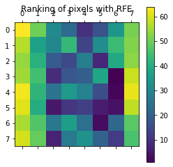
from sklearn.svm import SVC
from sklearn.datasets import load_digits
from sklearn.feature_selection import RFE
import matplotlib.pyplot as plt

# Load the digits dataset
digits = load_digits()
X = digits.images.reshape((len(digits.images), -1))
y = digits.target
print("variable X Dimensions:")
print(X.shape)

# Create the RFE object and rank each pixel
svc = SVC(kernel="linear", C=1)
rfe = RFE(estimator=svc, n_features_to_select=1, step=1)
rfe.fit(X, y)
ranking = rfe.ranking_.reshape(digits.images[0].shape)
print("variable ranking Dimensions:")
print(ranking.shape)

# Plot pixel ranking
plt.matshow(ranking)
plt.colorbar()
plt.title("Ranking of pixels with RFE")
plt.show()

The dimension of variable X:
(1797, 64)
The dimension of ranking of variables:
(8, 8)

4. SelectFromModel

First, SelectFromModel is proposed to process data from Model. If the relevant coef_or feature portals attribute values are lower than the preset threshold, these features will be considered unimportant and removed. In addition to being able to specify thresholds, you can also find an appropriate threshold by using built-in heuristic methods with given string parameters.

• Example

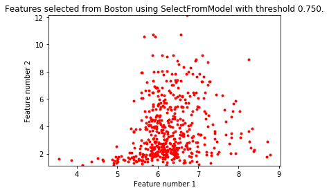
import matplotlib.pyplot as plt
import numpy as np

from sklearn.datasets import load_boston
from sklearn.feature_selection import SelectFromModel
from sklearn.linear_model import LassoCV

# Load the boston dataset.
boston = load_boston()
X, y = boston['data'], boston['target']

# We use the base estimator LassoCV since the L1 norm promotes sparsity of features.
clf = LassoCV(cv=5)

# Set a minimum threshold of 0.25
sfm = SelectFromModel(clf, threshold=0.25)
sfm.fit(X, y)
n_features = sfm.transform(X).shape[1]

# Modify threshold value
while n_features > 2:
    sfm.threshold += 0.1
    X_transform = sfm.transform(X)
    n_features = X_transform.shape[1]

# Drawing scatter plots of two characteristic variables from X
plt.title(
    "Features selected from Boston using SelectFromModel with "
    "threshold %0.3f." % sfm.threshold)
feature1 = X_transform[:, 0]
feature2 = X_transform[:, 1]
print("variable X Dimensions:")
print(X.shape)
print("Dimensions of selected data:")
print(X_transform.shape)
plt.plot(feature1, feature2, 'r.')
plt.xlabel("Feature number 1")
plt.ylabel("Feature number 2")
plt.ylim([np.min(feature2), np.max(feature2)])
plt.show()

The dimension of variable X:
(506, 13)
Dimensions of selected data:
(506, 2)

4.1 Feature Selection Based on L 1

Linear models use L1 regularized linear models to get sparse solutions: many of their coefficients are zero.

from sklearn.svm import LinearSVC
from sklearn.datasets import load_iris
from sklearn.feature_selection import SelectFromModel
iris = load_iris()
X, y = iris.data, iris.target
print("X.shape")
print(X.shape)
lsvc = LinearSVC(C=0.01, penalty="l1", dual=False).fit(X, y)
model = SelectFromModel(lsvc, prefit=True)
X_new = model.transform(X)
print("X_new.shape")
print(X_new.shape)

X.shape
(150, 4)
X_new.shape
(150, 3)

4.2 Tree-based feature selection

Tree-based feature selection can be used to calculate the importance of features, and then irrelevant features can be eliminated.

• Example

from sklearn.ensemble import ExtraTreesClassifier
from sklearn.datasets import load_iris
from sklearn.feature_selection import SelectFromModel
iris = load_iris()
X, y = iris.data, iris.target
print("X.shape")
print(X.shape)
clf = ExtraTreesClassifier()
clf = clf.fit(X, y)
print("clf.feature_importances_")
print(clf.feature_importances_)
model = SelectFromModel(clf, prefit=True)
X_new = model.transform(X)
print("X_new.shape")
print(X_new.shape)

X.shape
(150, 4)
clf.feature_importances_
[0.03024885 0.04546254 0.43126586 0.49302275]
X_new.shape
(150, 2)

5. Feature selection as part of pipeline

Feature selection is usually used for preprocessing before actual learning. The recommended approach in scikit-learn s is to use sklearn.pipeline.Pipeline

clf = Pipeline([
  ('feature_selection', SelectFromModel(LinearSVC(penalty="l1"))),
  ('classification', RandomForestClassifier())
])
clf.fit(X, y)

In this code, we use sklearn.svm.LinearSVC and sklearn.feature_selection.SelectFromModel to evaluate the importance of features and select the relevant features. Then, a sklearn.ensemble.RandomForestClassifier classifier is used in the transformed output, such as using only relevant features.