This learning note is the learning content of Alibaba cloud Tianchi Longzhu data mining training camp. The learning links are: -Tianchi Lab - a real-time online data analysis collaboration tool, enjoy free computing resources (aliyun.com)

1, Summary of learning points

• Further analyze the features and process the data

• Complete the analysis of Feature Engineering, and make some charts or text summary for the data.

2, Learning content

1. Exception handling:
   • Delete outliers through box diagram (or 3-Sigma) analysis;
   • BOX-COX conversion (processing biased distribution);
   • Long tail truncation;
2. Feature normalization / standardization:
   • Standardization (conversion to standard normal distribution);
   • Normalization (switching to [0,1] interval);
   • For power-law distribution, the formula can be used:   log(1+x/1+median)
3. Data bucket:
   • Equal frequency bucket;
   • Equidistant barrel separation;
   • Best KS bucket classification (similar to secondary classification using Gini index);
   • Chi square barrel separation;
4. Missing value handling:
   • No processing (for tree models such as XGBoost);
   • Delete (too much missing data);
   • Interpolation completion, including mean / median / mode / modeling prediction / multiple interpolation / compressed sensing completion / matrix completion, etc;
   • Sub box, one box missing value;
5. Feature construction:
   • Construct statistical features, report counting, summation, proportion, standard deviation, etc;
   • Time characteristics, including relative time and absolute time, holidays, weekends, etc;
   • Geographic information, including box division, distribution coding and other methods;
   • Nonlinear transformation, including log / square / root sign, etc;
   • Feature combination, feature intersection;
   • Benevolent people see benevolence, wise people see wisdom.
6. Feature screening
   • filter: first select the characteristics of the data, and then train the learner. The common methods are Relief / variance selection / correlation coefficient method / chi square test / mutual information method;
   • Wrapper: directly take the performance of the learner to be used as the evaluation criterion of the feature subset. The common methods are LVM (Las Vegas Wrapper);
   • embedding: combining filtering and wrapping, feature selection is automatically carried out in the process of learner training. The common ones are lasso regression;
7. Dimensionality reduction
   • PCA/ LDA/ ICA；
   • Feature selection is also a dimension reduction.

(1) Delete outliers

# Here I wrap an exception handling code, which can be called at will.
def outliers_proc(data, col_name, scale=3):
    """
    Used to clean outliers. It is used by default box_plot(scale=3)Clean
    :param data: receive pandas data format
    :param col_name: pandas Listing
    :param scale: scale
    :return:
    """

    def box_plot_outliers(data_ser, box_scale):
        """
        Remove outliers using box diagram
        :param data_ser: receive pandas.Series data format
        :param box_scale: Dimension of box diagram,
        :return:
        """
        iqr = box_scale * (data_ser.quantile(0.75) - data_ser.quantile(0.25))
        val_low = data_ser.quantile(0.25) - iqr
        val_up = data_ser.quantile(0.75) + iqr
        rule_low = (data_ser < val_low)
        rule_up = (data_ser > val_up)
        return (rule_low, rule_up), (val_low, val_up)

    data_n = data.copy()
    data_series = data_n[col_name]
    rule, value = box_plot_outliers(data_series, box_scale=scale)
    index = np.arange(data_series.shape[0])[rule[0] | rule[1]]
    print("Delete number is: {}".format(len(index)))
    data_n = data_n.drop(index)
    data_n.reset_index(drop=True, inplace=True)
    print("Now column number is: {}".format(data_n.shape[0]))
    index_low = np.arange(data_series.shape[0])[rule[0]]
    outliers = data_series.iloc[index_low]
    print("Description of data less than the lower bound is:")
    print(pd.Series(outliers).describe())
    index_up = np.arange(data_series.shape[0])[rule[1]]
    outliers = data_series.iloc[index_up]
    print("Description of data larger than the upper bound is:")
    print(pd.Series(outliers).describe())
    
    fig, ax = plt.subplots(1, 2, figsize=(10, 7))
    sns.boxplot(y=data[col_name], data=data, palette="Set1", ax=ax[0])
    sns.boxplot(y=data_n[col_name], data=data_n, palette="Set1", ax=ax[1])
    return data_n

# We can delete some abnormal data, taking power as an example.  
# Students can decide whether to delete it or not
# However, it should be noted that the data of test cannot be deleted = = can't hide your ears, can't you

train = outliers_proc(train, 'power', scale=3)

(2) Characteristic structure

# The training set and test set are put together to facilitate the construction of features
train['train']=1
test['train']=0
data = pd.concat([train, test], ignore_index=True, sort=False)

# Usage time: data ['createdate '] - Data ['regdate'], which reflects the usage time of the car. Generally speaking, the price is inversely proportional to the usage time
# However, note that there are time error formats in the data, so we need errors='coerce '
data['used_time'] = (pd.to_datetime(data['creatDate'], format='%Y%m%d', errors='coerce') - 
                            pd.to_datetime(data['regDate'], format='%Y%m%d', errors='coerce')).dt.days

# Look at the empty data. There is a problem with the time of 15k samples. We can choose to delete or put them.
# However, deletion is not recommended here because deletion of missing data accounts for 7.5% of the total sample size
# We can put it first, because if we use a decision tree such as XGBoost, it can handle missing values, so we can ignore it;
data['used_time'].isnull().sum()

15072

# Extracting city information from the zip code is German data, so referring to the zip code of Germany is equivalent to adding a priori knowledge
data['city'] = data['regionCode'].apply(lambda x : str(x)[:-3])





# Calculate the sales statistics of a brand. Students can also calculate the statistics of other characteristics
# Here, the statistics are calculated based on the data of train
train_gb = train.groupby("brand")
all_info = {}
for kind, kind_data in train_gb:
    info = {}
    kind_data = kind_data[kind_data['price'] > 0]
    info['brand_amount'] = len(kind_data)
    info['brand_price_max'] = kind_data.price.max()
    info['brand_price_median'] = kind_data.price.median()
    info['brand_price_min'] = kind_data.price.min()
    info['brand_price_sum'] = kind_data.price.sum()
    info['brand_price_std'] = kind_data.price.std()
    info['brand_price_average'] = round(kind_data.price.sum() / (len(kind_data) + 1), 2)
    all_info[kind] = info
brand_fe = pd.DataFrame(all_info).T.reset_index().rename(columns={"index": "brand"})
data = data.merge(brand_fe, how='left', on='brand')

  Data bucket

# Data bucket Division: take power as an example
# At this time, our missing values are also in the bucket,
# There are many reasons why data buckets should be divided, ==
# 1. After discretization, the multiplication of sparse vector inner product is faster, and the calculation results are easy to store and expand;
# 2. The features after discretization are more robust to outliers, such as age > 30 is 1, otherwise it is 0, and it will not cause great interference to the model when the age is 200;
# 3. LR is a generalized linear model with limited expression ability. After discretization, each variable has a separate weight, which is equivalent to the introduction of nonlinearity, which can improve the expression ability of the model and increase the fitting;
# 4. After discretization, the features can be crossed to improve the expression ability. M*N variables are programmed by M+N variables, and non-linear is further introduced to improve the expression ability;
# 5. After feature discretization, the model is more stable, such as the user's age range, which will not change because the user's age is one year older

# Of course, there are many reasons. When improving XGBoost, LightGBM adds data buckets to enhance the generalization of the model

bin = [i*10 for i in range(31)]
data['power_bin'] = pd.cut(data['power'], bin, labels=False)
data[['power_bin', 'power']].head()

#If you make good use of it, you can delete the original data
data = data.drop(['creatDate', 'regDate', 'regionCode'], axis=1)

print(data.shape)
data.columns

 

(199037, 39)

[15]:

Index(['SaleID', 'name', 'model', 'brand', 'bodyType', 'fuelType', 'gearbox',
,       'power', 'kilometer', 'notRepairedDamage', 'seller', 'offerType',
,       'price', 'v_0', 'v_1', 'v_2', 'v_3', 'v_4', 'v_5', 'v_6', 'v_7', 'v_8',
,       'v_9', 'v_10', 'v_11', 'v_12', 'v_13', 'v_14', 'train', 'used_time',
,       'city', 'brand_amount', 'brand_price_average', 'brand_price_max',
,       'brand_price_median', 'brand_price_min', 'brand_price_std',
,       'brand_price_sum', 'power_bin'],
,      dtype='object')

# The current data can actually be used for the tree model, so let's export it
data.to_csv('data_for_tree.csv', index=0)

# We can construct another feature for models such as LR and NN
# The reason why they are constructed separately is that different models have different requirements for data sets
# Let's look at the data distribution:
data['power'].plot.hist()

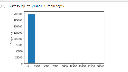
 # We have just handled the outliers of train, but now there is such a strange distribution because of the power outliers in test,
#Therefore, it is better not to delete the power outliers in the train, which can be replaced by long tailed distribution truncation
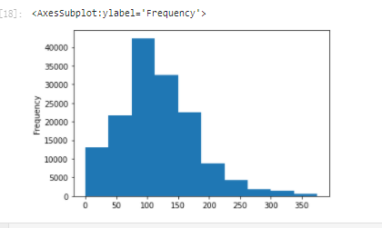
train['power'].plot.hist()

 

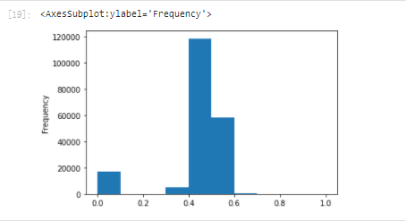
# We take the log and normalize it
from sklearn import preprocessing
min_max_scaler = preprocessing.MinMaxScaler()
data['power'] = np.log(data['power'] + 1) 
data['power'] = ((data['power'] - np.min(data['power'])) / (np.max(data['power']) - np.min(data['power'])))
data['power'].plot.hist()

 

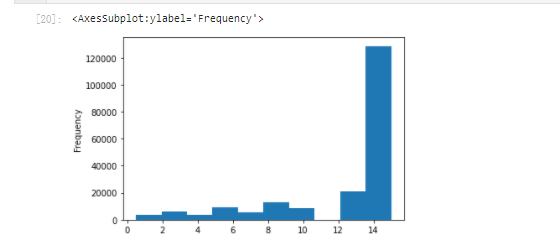
# km is quite normal. It should have been done too much
data['kilometer'].plot.hist()

 

# So we can do normalization directly
data['kilometer'] = ((data['kilometer'] - np.min(data['kilometer'])) / 
                        (np.max(data['kilometer']) - np.min(data['kilometer'])))
data['kilometer'].plot.hist()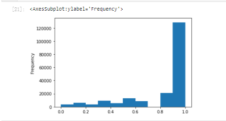

 

# In addition, there are the statistical features we have just constructed:
# 'brand_amount', 'brand_price_average', 'brand_price_max',
# 'brand_price_median', 'brand_price_min', 'brand_price_std',
# 'brand_price_sum'
# There are no more examples to analyze one by one here. Just do the transformation,
def max_min(x):
    return (x - np.min(x)) / (np.max(x) - np.min(x))

data['brand_amount'] = ((data['brand_amount'] - np.min(data['brand_amount'])) / 
                        (np.max(data['brand_amount']) - np.min(data['brand_amount'])))
data['brand_price_average'] = ((data['brand_price_average'] - np.min(data['brand_price_average'])) / 
                               (np.max(data['brand_price_average']) - np.min(data['brand_price_average'])))
data['brand_price_max'] = ((data['brand_price_max'] - np.min(data['brand_price_max'])) / 
                           (np.max(data['brand_price_max']) - np.min(data['brand_price_max'])))
data['brand_price_median'] = ((data['brand_price_median'] - np.min(data['brand_price_median'])) /
                              (np.max(data['brand_price_median']) - np.min(data['brand_price_median'])))
data['brand_price_min'] = ((data['brand_price_min'] - np.min(data['brand_price_min'])) / 
                           (np.max(data['brand_price_min']) - np.min(data['brand_price_min'])))
data['brand_price_std'] = ((data['brand_price_std'] - np.min(data['brand_price_std'])) / 
                           (np.max(data['brand_price_std']) - np.min(data['brand_price_std'])))
data['brand_price_sum'] = ((data['brand_price_sum'] - np.min(data['brand_price_sum'])) / 
                           (np.max(data['brand_price_sum']) - np.min(data['brand_price_sum'])))

# OneEncoder for category features
data = pd.get_dummies(data, columns=['model', 'brand', 'bodyType', 'fuelType',
                                     'gearbox', 'notRepairedDamage', 'power_bin'])

print(data.shape)
data.columns

(199037, 370)

[24]:

Index(['SaleID', 'name', 'power', 'kilometer', 'seller', 'offerType', 'price',
,       'v_0', 'v_1', 'v_2',
,       ...
,       'power_bin_20.0', 'power_bin_21.0', 'power_bin_22.0', 'power_bin_23.0',
,       'power_bin_24.0', 'power_bin_25.0', 'power_bin_26.0', 'power_bin_27.0',
,       'power_bin_28.0', 'power_bin_29.0'],
,      dtype='object', length=370)

# This data can be used by LR
data.to_csv('data_for_lr.csv', index=0)

(3) Feature screening

1) Filter type

# correlation analysis 
print(data['power'].corr(data['price'], method='spearman'))
print(data['kilometer'].corr(data['price'], method='spearman'))
print(data['brand_amount'].corr(data['price'], method='spearman'))
print(data['brand_price_average'].corr(data['price'], method='spearman'))
print(data['brand_price_max'].corr(data['price'], method='spearman'))
print(data['brand_price_median'].corr(data['price'], method='spearman'))

0.5728285196051496

-0.4082569701616764

0.058156610025581514

0.3834909576057687

0.259066833880992

0.38691042393409447

# Of course, you can also look at the picture directly
data_numeric = data[['power', 'kilometer', 'brand_amount', 'brand_price_average', 
                     'brand_price_max', 'brand_price_median']]
correlation = data_numeric.corr()

f , ax = plt.subplots(figsize = (7, 7))
plt.title('Correlation of Numeric Features with Price',y=1,size=16)
sns.heatmap(correlation,square = True,  vmax=0.8)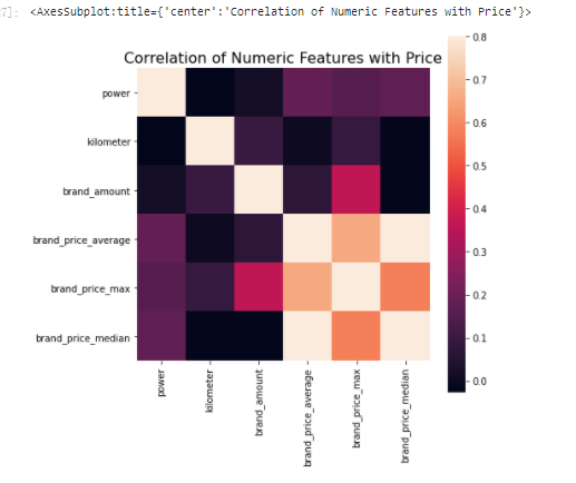

  (2) Wrapped

!pip install mlxtend

# k_ The feature is too large to run. There is no server, so interrupt in advance
from mlxtend.feature_selection import SequentialFeatureSelector as SFS
from sklearn.linear_model import LinearRegression
sfs = SFS(LinearRegression(),
           k_features=10,
           forward=True,
           floating=False,
           scoring = 'r2',
           cv = 0)
x = data.drop(['price'], axis=1)
numerical_cols = x.select_dtypes(exclude = 'object').columns
x = x[numerical_cols]
x = x.fillna(0)
y = data['price'].fillna(0)
sfs.fit(x, y)
sfs.k_feature_names_ 

('kilometer',
, 'v_0',
, 'v_3',
, 'v_7',
, 'train',
, 'used_time',
, 'brand_price_average',
, 'brand_price_std',
, 'model_167.0',
, 'gearbox_1.0')

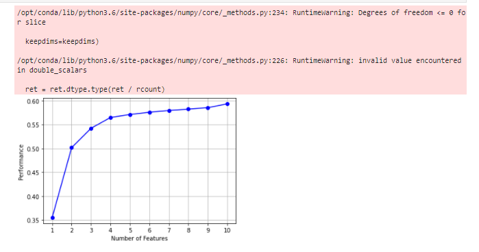
# Draw it and you can see the marginal benefit
from mlxtend.plotting import plot_sequential_feature_selection as plot_sfs
import matplotlib.pyplot as plt
fig1 = plot_sfs(sfs.get_metric_dict(), kind='std_dev')
plt.grid()
plt.show()

  3) Embedded

#The next chapter introduces that Lasso regression and decision tree can complete embedded feature selection
#In most cases, embedded is used for feature filtering

3, Learning questions and answers

Structural features are essentially the relationship between structural features and predicted values. Several more features can be constructed to enhance the accuracy of the model.

The main purpose of feature engineering is to transform data into features that can better represent potential problems, so as to improve the performance of machine learning. For example, outlier processing is to remove noise, fill in missing values, and add a priori knowledge.

4, Learning, thinking and summary

Some competitions are characterized by anonymous features, which makes us not clear the direct correlation between features. At this time, we can only process based on features, such as boxing, groupby, agg, etc. for some feature statistics. In addition, we can further transform the features such as log and exp, or perform four operations on multiple features (such as the usage time calculated above), polynomial combination, etc., and then filter. Because of the anonymity of the feature, it actually limits a lot of feature processing. Of course, sometimes using NN to extract some features will also achieve unexpected good results.

For those who know the meaning of the feature (not anonymous) Feature Engineering, especially in the industrial type competition, will build more practical features based on signal processing, frequency domain extraction, abundance, skewness, etc., which is the feature construction combined with the background, and the same is true in the recommendation system. Such a feature construction often needs to be deeply divided into various types of click through rate statistics, statistics of each period, statistics of user attributes, etc Analyze the business logic or physical principles behind it, so as to better find magic.

Of course, feature engineering is actually combined with the model, which is why it is necessary to divide buckets and normalize features for LR NN, and the processing effect and importance of features are often verified by the model.

In general, feature engineering is a simple entry, but it is very difficult to master it.