1, Using excel to do linear regression

1. Startup steps

Find data analysis in the data column of excel, and then start linear regression. If there is no "data analysis" tab, you can select "add in" in the "file" tab and select "go" as follows:

Check the required tool

2. Data analysis

After importing the height and weight data set, collect the first 20 items for data analysis, and the following results can be obtained:

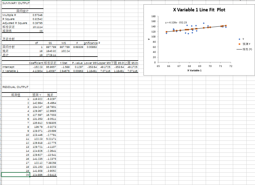
• Correlation coefficient (Multiple): 0.570
• P-value: 0.01 < p < 0.005, so the regression equation is established.
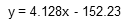
  The linear regression equation is
  
  Next, take a look at the first 200 items
  
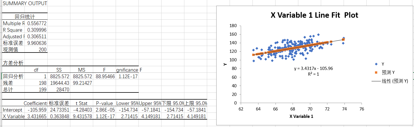
• Multiple: 0.556
• P-value: 0.01 < p < 0.005, so the regression equation is established.
  The linear regression equation is
  
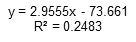
  The first two thousand groups of data:
  
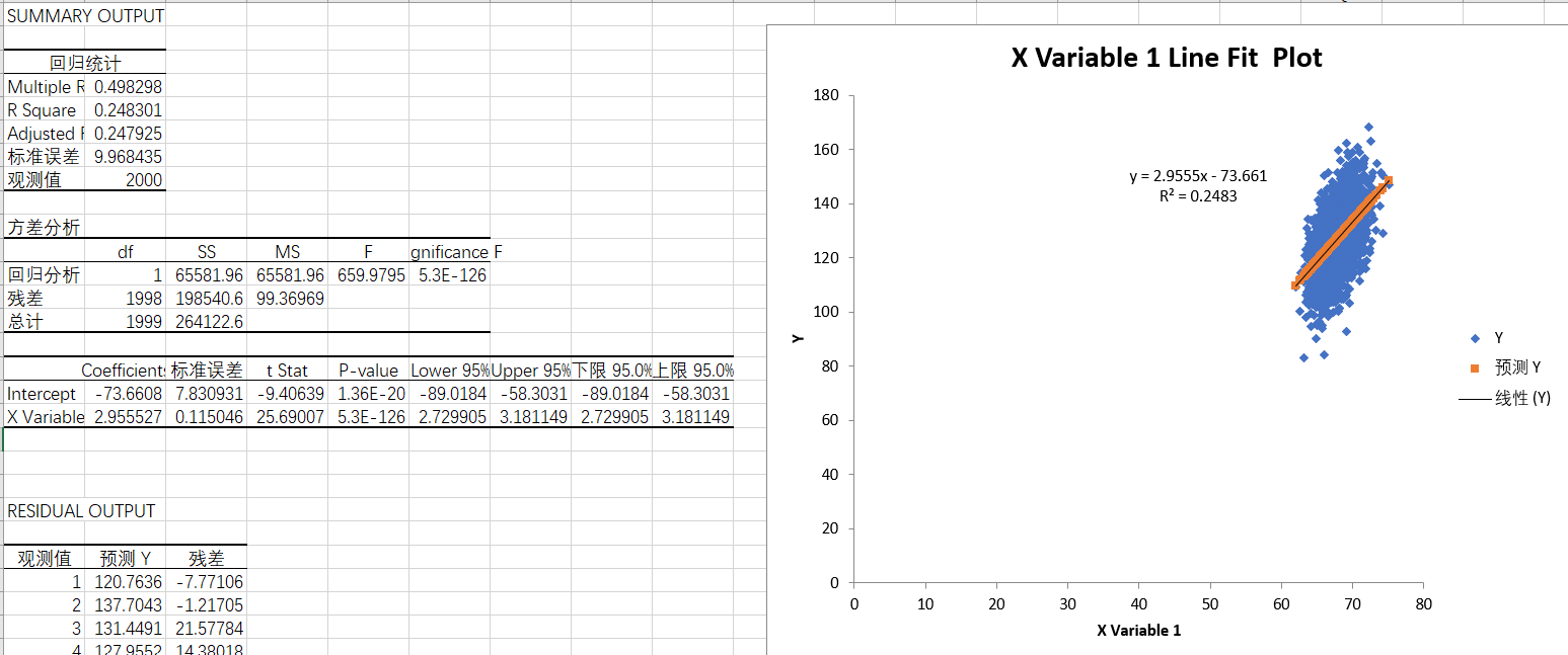
• Multiple: 0.498
• P-value: 0.01 < p < 0.005, so the regression equation is established.
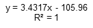
  The linear regression equation is
  
  It can be seen that when there is more data, the value of R^2 changes greatly

2, jupyter programming

1. Data import

After downloading the software, open

The following interface will appear

This interface is used to connect the web and your local machine. It cannot be closed during use.
The software will automatically open and import our data set (Note: click upload after import)

2. Least square coding without third-party library

Enter the following code in the new python file:

import pandas as pd
import numpy as np
import math
#Prepare data
p=pd.read_excel('weights_heights(height-Weight data set).xls','weights_heights')
#Add according to your needs. Here, select the first 20 rows of data
p1=p.head(20)
x=p1["Height"]
y=p1["Weight"]
# average value
x_mean = np.mean(x)
y_mean = np.mean(y)
#Total number of x (or y) columns (i.e. n)
xsize = x.size
zi=((x-x_mean)*(y-y_mean)).sum()
mu=((x-x_mean)*(x-x_mean)).sum()
n=((y-y_mean)*(y-y_mean)).sum()
# Parameters a and B
a = zi / mu
b = y_mean - a * x_mean
#Square of correlation coefficient R
m=((zi/math.sqrt(mu*n))**2)
# Here, 4 significant digits are reserved for parameters
a = np.around(a,decimals=4)
b = np.around(b,decimals=4)
m = np.around(m,decimals=4)
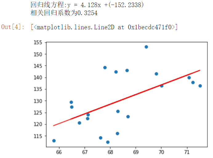
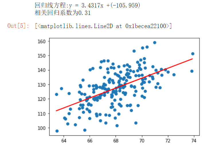
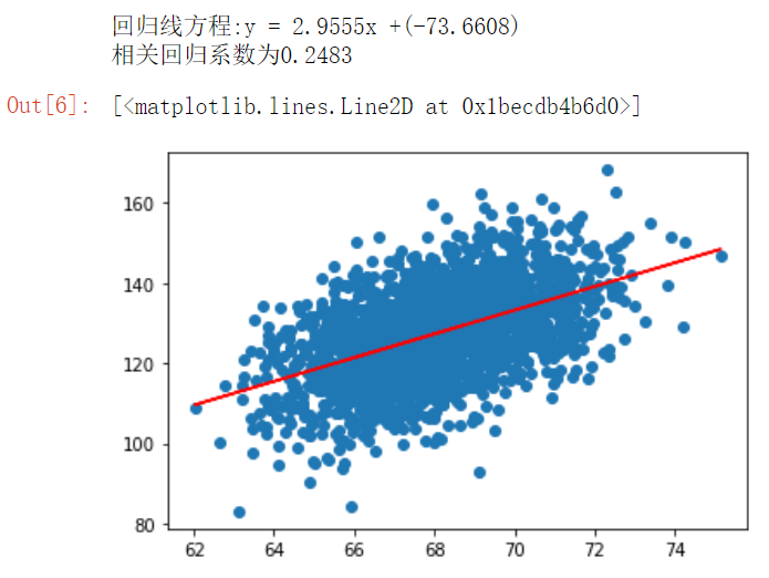
print(f'Regression line equation:y = {a}x +({b})') 
print(f'The correlation regression coefficient is{m}')
#Draw the fitting curve with the help of the third-party library skleran
y1 = a*x + b
plt.scatter(x,y)
plt.plot(x,y1,c='r')

The following are the test results
Top 20 data results

Top 200 data results

First 2000 data results

3. Use skleran coding

The code is as follows:

# Import required modules
import numpy as np
import pandas as pd
import matplotlib.pyplot as plt
from sklearn.linear_model import LinearRegression

p=pd.read_excel('weights_heights(height-Weight data set).xls','weights_heights')
#Number of data rows read
p1=p.head(20)
x=p1["Height"]
y=p1["Weight"]
# data processing
# The input and output of sklearn fitting are generally two-dimensional arrays. Here, one dimension is transformed into two dimensions.
y = np.array(y).reshape(-1, 1)
x = np.array(x).reshape(-1, 1)
# fitting
reg = LinearRegression()
reg.fit(x,y)
a = reg.coef_[0][0]     # coefficient
b = reg.intercept_[0]   # intercept
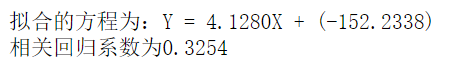
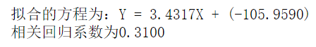
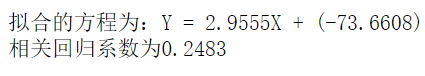
print('The fitted equation is: Y = %.4fX + (%.4f)' % (a, b))
c=reg.score(x,y)    # correlation coefficient
print(f'The correlation regression coefficient is%.4f'%c)

# visualization
prediction = reg.predict(y)                
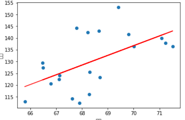
plt.xlabel('height')
plt.ylabel('weight')
plt.scatter(x,y)
y1 = a*x + b
plt.plot(x,y1,c='r')

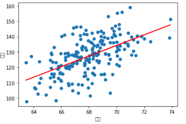
Top 20 groups of data


First 200 groups of data


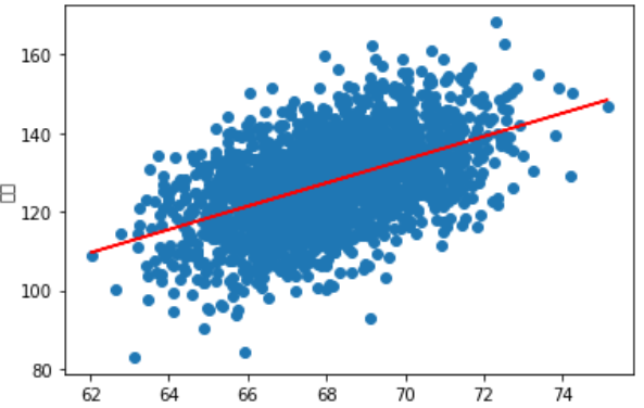
First 2000 groups of data

3, Summary

The results of the three methods are similar. Although excel is convenient and easy, using jupyter is more helpful for us to understand the internal algorithm of machine learning and the related knowledge of linear regression.