catalogue
Brief introduction of Markowitz model
② The combination weight is calculated by Monte Carlo method
③ Select the effective frontier combination
④ Stock performance during the test period
⑤ Returns of effective frontier portfolio in the test period
Brief introduction of Markowitz model
1, Principle
Markowitz mean variance portfolio model is simply to make the portfolio with the smallest variance at a specific level of return.
Implicit conditions: ① invest in multiple stocks to spread risks; ② The correlation coefficient between stocks is low.
2, Correlation formula
Revenue vector 
Expectation vector
Variance vector
Covariance matrix
Weight vector
Portfolio income
Combination expectation
Combined variance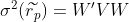
Specific reference: Financial mathematics Chapter III mean variance portfolio selection model - MBA think tank document
Example verification
1, Method selection
The combined effective frontier can be solved by quadratic programming. In this example, Monte Carlo simulation is selected, that is, a large number of random operators are put into simulation.
2, Train of thought
Use the data of a period of time to calculate the effective frontier weight of the portfolio, and use this weight to calculate the return in the subsequent period of time.
① Assumptions
The earnings of the selected stocks in the calculation period are positive, assuming that they have a continuous upward trend in the following period of time.
② Set
The calculation time period is 3 months, and the test (prediction) time period is the latest (about 1.5 months).
③ Attention
The selected stocks need low correlation to better disperse the risk this time.
3, Practice
① Data preparation
Stocks are found at random. If they meet the assumptions, they are ok and do not constitute investment suggestions.
If you want to customize the program, please send a private letter, thank you!
# Prepare stock code
stock_list = ['600176.SH',\
'002594.SZ',\
'002080.SZ',\
'000733.SZ',\
'600373.SH',\
'300142.SZ',\
'300498.SZ',\
'002625.SZ',\
'000519.SZ',\
'603290.SH',\
'300502.SZ']
# Set the time period for preparing data
# Data time period used for calculation
start_date_cal = '20210701'
end_date_cal = '20210930'
# Data period used as test
start_date_test = '20211001'
end_date_test = '20211115'
# Get the price of each stock
stock_price = get_stock_price(stock_list, start_date_cal, end_date_cal) # Data for calculation
stock_price_test = get_stock_price(stock_list, start_date_test, end_date_test) # Data for testing
# Starting from 1, the difference can be seen more intuitively
stock_price_1 = dfUnification(stock_price) # Data for calculation
stock_price_1_test = dfUnification(stock_price_test) # Data for testing
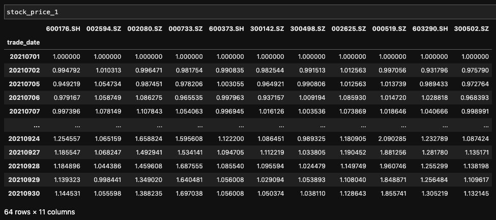
# Calculate the daily return of each stock
stock_daily_returns = getDailyReturns(stock_price)
stock_daily_returns_test = getDailyReturns(stock_price_test)
# Calculate correlation matrix
correlation_matrix = stock_daily_returns.corr()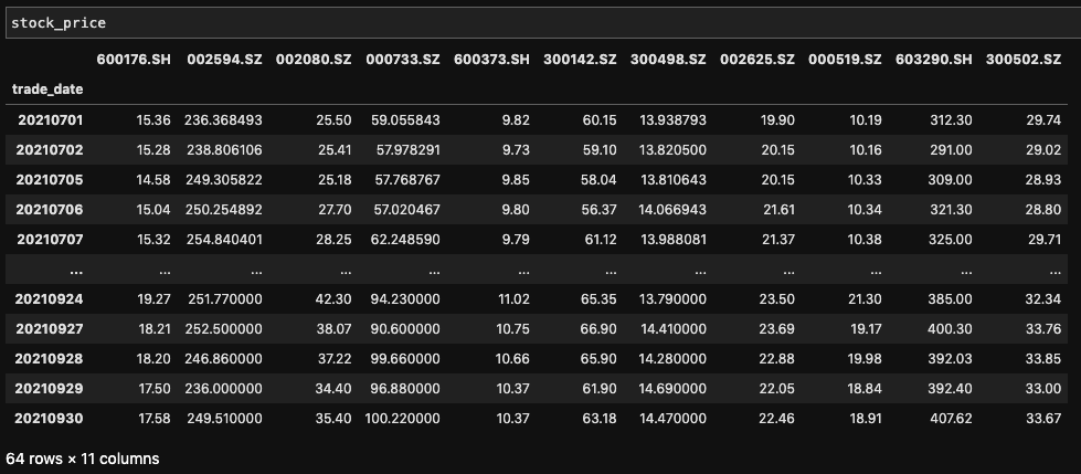
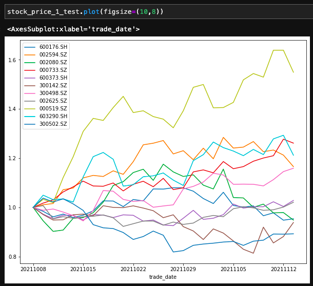
 The trend of the stock in the calculation period is as follows (the initial net value is 1, which can better see the trend)
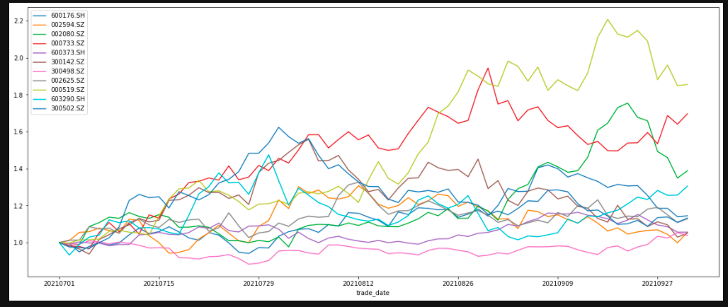
# Thermodynamic diagram of correlation coefficient between stocks
sns.heatmap(correlation_matrix,annot=True,cmap='rainbow',linewidths=1.0,annot_kws={'size':8})
plt.xticks(rotation=45)
plt.yticks(rotation=0)
plt.show()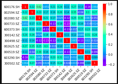
② The combination weight is calculated by Monte Carlo method
The Returns calculated here is the compound annualized rate of return with the daily average rate of return.
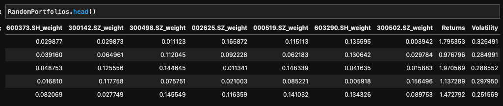
RandomPortfolios = monteCarloTest(stock_daily_returns)

#Scatter plot
RandomPortfolios.plot('Volatility','Returns',kind='scatter',alpha=0.3)
plt.show() 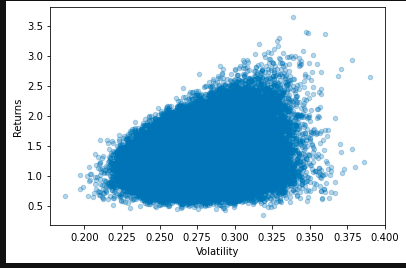
③ Select the effective frontier combination
Because there are a lot of decimal places in Returns, if the decimal places are reduced, then when the Returns values are equal, selecting the minimum Volatility vertically is equivalent to selecting the combination of effective frontier.
RandomPortfolios['ReturnsRound'] = round(RandomPortfolios.Returns, 2)
returns_range = pd.DataFrame(sorted(RandomPortfolios['ReturnsRound'])).drop_duplicates()[0].tolist()
vol_min_idx_l = []
for i in returns_range:
    vol_min = RandomPortfolios[RandomPortfolios['ReturnsRound']==i].Volatility.min()
    vol_min_idx = RandomPortfolios[RandomPortfolios['Volatility']==vol_min].index[0]
    vol_min_idx_l.append(vol_min_idx)

RandomPortfolios.loc[vol_min_idx_l].plot('Volatility','Returns',kind='scatter',alpha=0.3)
plt.show()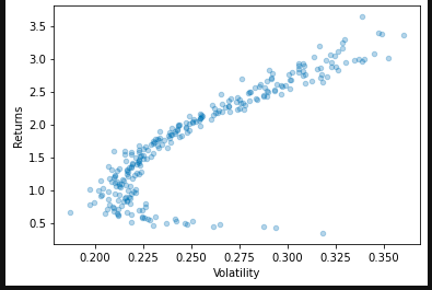
④ Stock performance during the test period
There are individual stocks that can fall.
⑤ Returns of effective frontier portfolio in the test period
Returns for the test period_ Note that it is not an annualized rate of return.
# Calculate the yield of random weight in the test period
Returns_test = []
for i in range(RandomPortfolios.shape[0]):
    Returns_test.append(stock_price_1_test.mul(\
                        np.array(RandomPortfolios.iloc[i,:stock_price_1_test.shape[1]]), axis=1).sum(axis=1).iloc[-1] - 1)

RandomPortfolios['Returns_test'] = Returns_test

plt.scatter(RandomPortfolios.loc[vol_min_idx_l].Volatility, RandomPortfolios.loc[vol_min_idx_l].Returns, c=RandomPortfolios.loc[vol_min_idx_l].Returns_test)
plt.colorbar(label='Returns_test')
plt.show()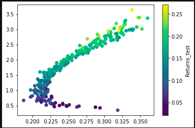
The return of effective frontier portfolio in the test period is still OK, and basically follows the relationship between risk and return.
4, Thinking
Is the result in this example individual or common? Can this strategy be replicated? Is it related to the selected calculation and test time period? If other time periods are selected, will there be consistent results? Is it also related to the selected stocks and the number of stocks in the portfolio?
The problem is left to ourselves and to everyone.
If you want to customize the program, please send a private letter, thank you!