Pan Chuang AI sharing

Author kajal56

Compile Flin

Source | analyticsvidhya

summary

We live in a digital world today. From the beginning of the day to saying "good night" to our loved ones, we consume a lot of data in the form of vision, music / audio, network, text and more sources.

Today, we will explore one of these data sources to see if we can get information from it.

Due to comments, feedback, articles and many other data collection / publishing methods, we will use a large number of available "text" data.

We'll try to see if we can capture "emotions" from a given text, but first, we'll preprocess and structure the given "text" data because it's an unstructured row form. We need to convert text data to structured format, because most machine learning algorithms use structured data.

In this article, we will use public data from "Kaggle". Please use the following link to get the data.

https://www.kaggle.com/amitkumardas/sentiment-train

This will be a classification exercise because the dataset consists of movie reviews from users marked as positive or negative.

Emotion classification

The dataset we just discussed contains movie reviews. Each comment is marked positive or negative. The dataset contains text and emotion fields. These fields are separated by tab characters. See below for details:

**1. text: * * sentence describing the comment.

2. sentiment: 1 or 0. 1 represents positive evaluation and 0 represents negative evaluation.

Now we will discuss the whole process of "emotion classification". The following is the process of the project.

1. Load dataset
2. Explore datasets
3. Text preprocessing
4. Construct emotion classification model
5. Split dataset
6. Predict test cases
7. Find model accuracy

Load dataset

Read using panda_ The CSV () method loads data as follows:

import pandas as pd
import numpy as np
import warnings
warnings.filterwarnings('ignore')
train_data = pd.read_csv('sentiment_train.csv')
train_data.head(5)

The first five records of loading data are shown in the table below.


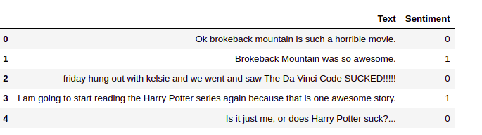
Because the default column width is limited, some text in the above table may have been truncated when obtaining the output. This can be done by setting max_colwidth parameter to increase the width size to change.

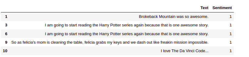
Each record or example in the column sentence is called a document. Use the following code to print the first five positive emotional documents.

pd.set_option('max_colwidth',1800)
train_data[train_data.label == 1][0:5]

The fifth positive emotion. An emotion value of 1 indicates positive emotion


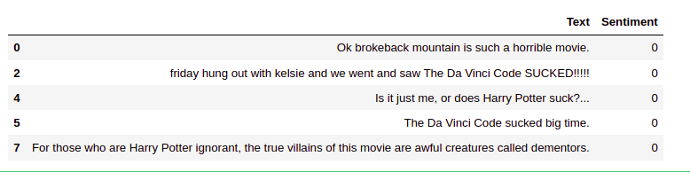
To print the first five negative emotion documents, use:

train_data[train_data.Sentiment == 1][0:5]

The first five negative emotions. An emotion value of 0 indicates negative emotion.


In the next section, we will discuss exploratory data analysis of text data.

Explore datasets

Exploratory data analysis can be carried out by counting the number of comments, positive comments, negative comments, etc. for example, how many comments can we view in the data set? Are the positive and negative emotional comments in the data set well reflected? Use the info() method to print the metadata of the data frame.

train_data.info()


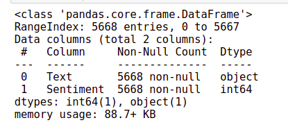
From the output, we can infer that there are 5668 records in the dataset. We created a count chart to compare the number of positive and negative emotions.

import matplotlib.pyplot as plt
import seaborn as sn
%matplotlib inline
plt.figure(figsize=(6,5))
plt.title("Number of records of positive and negative sentiments")
plot = sn.countplot(x = 'Sentiment', data=train_data)
for p in plot.patches:
    plot.annotate(p.get_height(),(p.get_x()+0.1 ,p.get_height()+50))


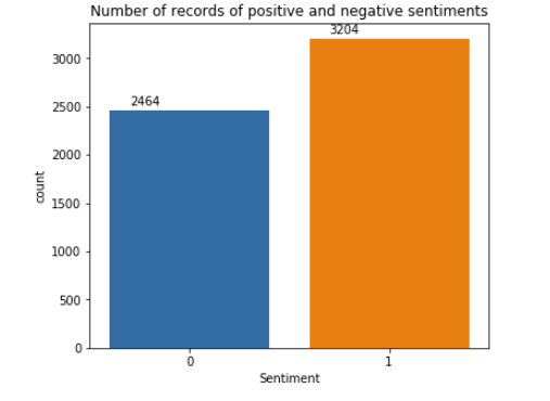
From the figure, we can infer that there are 5668 records in the dataset. Of the 5668 records, 2464 were negative emotions and 3204 were positive emotions. Therefore, positive and negative emotional documents have quite the same representation in the data set.

Before building the model, text data needs to be preprocessed for feature extraction. The following sections will introduce the text preprocessing technology step by step.

Text preprocessing

This section focuses on how to preprocess text data. Which function must be used to get a better dataset format that can apply the model to the text dataset.

We have some technology to complete this process. This article only discusses using to create count vectors. You can follow my other article to learn about other preprocessing techniques for text datasets.

Click here: https://www.analyticsvidhya.com/blog/2021/08/text-preprocessing-techniques-for-performing-sentiment-analysis/#h2_ three

All quantizer classes take the list of stop words as parameters and delete stop words when building dictionaries or feature sets. And these words do not appear in the count vector representing the document. We will bypass the stop word list to create a new count vector.

count_vectorizer =  CountVectorizer(stop_words= my_stop_words, max_features= 1000)

feature_vector =  count_vectorizer.fit(train_data.Text)

train_ds_features =  count_vectorizer.transform(train_data.Text)

features = feature_vector.get_feature_names()

features_counts = np.sum(train_ds_features.toarray(), axis = 0)

features_counts = pd.DataFrame(dict(features =  features, counts = features_counts))

features_counts.sort_values("counts", ascending= False)[0:15]

It can be noted that the stop words have been deleted. But we also noticed another problem. Many take many forms. For example, love and love. The vectorizer treats the two words as separate words, so it creates two separate features. But if all forms of a word have similar meanings, we can only use the root as the feature. Stem extraction and form reduction are two popular techniques for converting words into roots.

1. Stem: this eliminates the difference between the inflected forms of a word and reduces each word to its root form. This is mainly done by cutting off the end of the word. One problem with streaming is that word segmentation may cause words not to belong to the vocabulary. Porter Stemmer and Lancaster Stemmer are two popular streaming media algorithms. They have rules on how to truncate words.

2. Word form reduction: this considers the morphological analysis of words. It uses a language dictionary to convert words into roots. For example, stem can not distinguish the differences between people, and word form restoration can restore these words to the original words.

from nltk.stem.snowball import PorterStemmer

stemmer = PorterStemmer()

analyzer = CountVectorizer().build_analyzer()

def stemmed_words(doc):

   stemmed_words = [stemmer.stem(w) for w in analyzer(doc)]

   non_stop_words = [word for word in stemmed_words if not in my_stop_words]

   return non_stop_words

Before creating the count vector, the CountVectorizer uses a custom parser for streaming and stops deleting words. Therefore, the custom function stemmed_words() is passed as the parser.

count_vectorizer =  CountVectorizer(stop_words= my_stop_words, max_features= 1000)

feature_vector =  count_vectorizer.fit(train_data.Text)

train_ds_features =  count_vectorizer.transform(train_data.Text)

features = feature_vector.get_feature_names()

features_counts = np.sum(train_ds_features.toarray(), axis = 0)

features_counts = pd.DataFrame(dict(features =  features, counts = features_counts))

features_counts.sort_values("counts", ascending= False)[0:15]

Print the first 15 words and their counts in descending order.


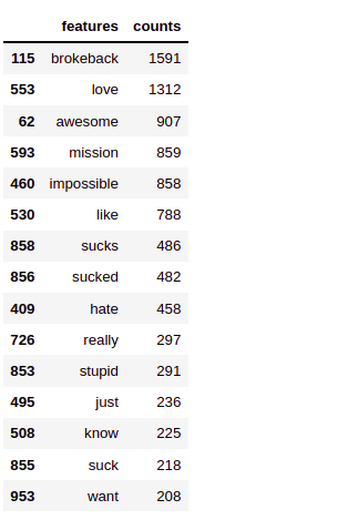
It can be noted that the words love, loved and awesome all come from the root.

After preprocessing, continue to build the model.

Establish emotion classification model

We will build different models to classify emotions.

1. Naive Bayes classifier
2. TF-IDF vectorizer

Now we will discuss them one by one.

Let's first discuss the naive Bayesian classifier

Naive Bayesian model for emotion classification

Naive Bayesian classifier is widely used in natural language processing and has been proved to provide better results. It applies to the concept of bayet's theorem.

Suppose we want to predict whether the probability of a document is positive, because the document contains a word awesome. This value can be calculated by multiplying the probability of the awesome word in the document with positive emotion by the probability of the document being positive.

P(doc = +ve | word = awesome) = P(word = awesome | doc = +ve) * P(doc = +ve)

The posterior probability of emotion is calculated from the prior probability of all words it contains. The assumption is that the words appearing in the document are considered independent and they do not affect each other.

Therefore, if the document contains N words and the words are expressed as w1, w2, w3,... wn, then

P(doc = +ve | word = w1, w2, w3.........wn) =

sklearn.naive_bayes provides a BernoulliNB class, which is a naive Bayesian classifier for multivariate BernoulliNB model. BernoulliNB is designed for binary features, which is the case here.

The steps of emotion classification using naive Bayesian model are as follows:

• Split the data set into training set and verification set,
• Establish a naive Bayesian model,
• Find model precision.

We will discuss these in the following sections.

Split the data set into training set and verification set

Use the following code to split the dataset into a ratio of 70:30 to create training and test datasets.

from sklearn.model_selection import train_test_split
train_x, test_x, train_y, test_y =  train_test_split(train_ds_features, train_data.Sentiment, 
                                                     test_size = 0.3, random_state = 42)

Constructing naive Bayesian model

The training set is used to construct the naive Bayesian model.

from sklearn.naive_bayes import BernoulliNB
nb_clf = BernoulliNB()
nb_clf.fit(train_x.toarray(), train_y)

Predict test cases

According to the calculation of naive Bayesian probability, the predicted category will be the category with high probability. The predicted test data set is evaluated using the predict() method.

test_ds_predicted = nb_clf.predict(test_x.toarray())

Find model accuracy

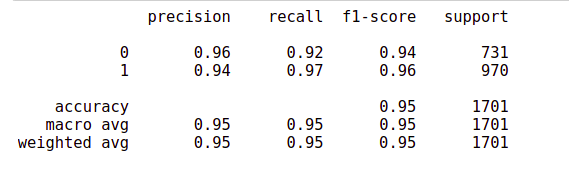
Let's print the classification report.

from sklearn import metrics
print(metrics.classification_report(test_y,test_ds_predicted))


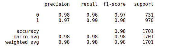
The model classifies with very high accuracy. The average accuracy and recall rate of identifying positive and negative emotional documents are about 98%. Let's draw the confusion matrix.

cm = metrics.confusion_matrix(test_y, test_ds_predicted)
sn.heatmap(cm, annot=True, fmt = '.2f')

In the confusion matrix, rows represent the actual number of positive and negative documents in the test set, while columns represent the content predicted by the model. Tag 1 indicates positive emotions and tag 0 indicates negative emotions.


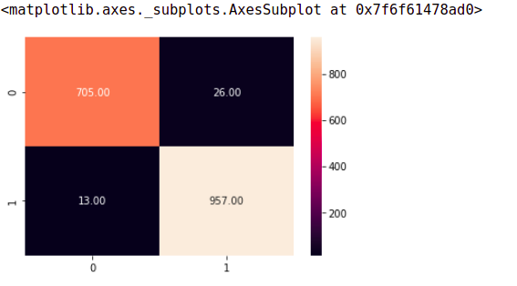
According to the model prediction, only 13 instances were incorrectly classified as negative emotion documents, and only 26 negative emotion documents were incorrectly classified as positive emotion documents. The rest have been correctly classified.

The next section will discuss the TD-IFD vectorization model.

**TF-IDF vectorizer**

Tfifvectorizer is used to create TF Vectorizer and TF-IDF Vectorizer. Use_ idf a parameter is required to create a TF-IDF vector. If used_ If idf is set to false, it will only create TF vectors. If set to True, it will create TF-IDF vectors.

from sklearn.feature_extraction.text import TfidfVectorizer
tfidf_vectorizer =  TfidfVectorizer(analyzer = stemmed_words, max_features = 1000)
feature_vector =  tfidf_vectorizer.fit(train_data.Text)
train_ds_features = tfidf_vectorizer.transform(train_data.Text)
features = feature_vector.get_feature_names()

TF IDF is a continuous value. It can be assumed that these continuous values associated with each class are distributed according to Gaussian distribution. Therefore, Gaussian naive Bayes can be used to classify these documents. We use Gaussian Nb, which implements Gaussian naive for classification_ Bayes algorithm.

from sklearn.naive_bayes import GaussianNB
train_x, test_x, train_y, test_y =  train_test_split(train_ds_features, train_data.Sentiment, 
                                                     test_size = 0.3, random_state = 42)

nb_clf = GaussianNB()
nb_clf.fit(train_x.toarray(), train_y)

test_ds_predicted =  nb_clf.predict(test_x.toarray())
print(metrics.classification_report(test_y,test_ds_predicted))


cm = metrics.confusion_matrix(test_y, test_ds_predicted)
sn.heatmap(cm, annot=True, fmt = '.2f')


The accuracy and recall rates seem to be almost the same. In this case, the accuracy is very high because the data set is clean and well planned. But this may not be the case in the real world.

conclusion

In this paper, text data is unstructured data, which needs a lot of preprocessing before applying the model. Naive Bayesian classification model is the most widely used text classification algorithm. The next article will discuss some of the challenges of text analysis using a small number of techniques, such as using N-Grams.